Control Engineering I · Week 12 · Damping Ratio and Natural Frequency of a Second-Order System

English translation

Edit the code and response fields in your own copy. Name: ⟦enter here⟧ / Student ID: ⟦enter here⟧

How to run

In Live Editor, click inside the code and run the current section with Run Section (Windows/Linux Ctrl+Enter, Mac ⌘+Enter). Run executes the entire document. Edit the explanations and response fields directly.

Initially run from the top, and rerun any section whose values you change. If an undefined-variable error occurs, run the preceding sections first. Outputs appear below or to the right of the code.

Environment: MATLAB Online and Control System Toolbox.

1. Calculate the performance conditions and design range

Perform the calculations below first, then compare with MATLAB results.

Change the code’s initial wn value from 4 to the value 5 specified for this activity.For the first run of the “4. Verify the design” code in the practice Live Script, use $\zeta=0.7,\quad\omega_n=5$ .
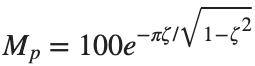
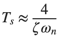
First calculate the overshoot and settling time by hand using $M_p=100e^{-\pi\zeta/\sqrt{1-\zeta^2}}$ [%] and $T_s\approx\frac{4}{\zeta\omega_n}$ .
Use $e^{-0.7\pi/\sqrt{0.51}}\approx0.046$ for numerical comparison.
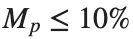
Determine whether $M_p\le10\%$ and $T_s\le2$ s are each satisfied. With $\zeta=0.7$ fixed, express the range of $\omega_n$ satisfying $T_s$ as an inequality.
Then change $\omega_n$ to 5 and run stepinfo to compare the approximation with the measured results.
Record this condition as one of the existing design combinations.

Before execution — Hand-calculated expressions and values: ⟦write calculations here⟧ After execution — MATLAB output values to compare: ⟦write output values here⟧

2. Convert to standard form

Start with K1=25,K2=4.

Prediction before running: ⟦enter here⟧

K1=25;K2=4;G=tf(K1,[1 K2 0]);T=feedback(G,1);
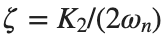
wn=sqrt(K1);zeta=K2/(2*wn);disp([wn,zeta]);
figure;step(T,0:.005:15);title(sprintf('wn=%.2f, zeta=%.2f',wn,zeta));grid on;
disp(stepinfo(T,'SettlingTimeThreshold',.02));

Do it yourself:

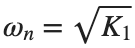
Calculate natural frequency $\omega_n=\sqrt{K_1}$ and damping ratio $\zeta=K_2/(2\omega_n)$ for the following two combinations: $(K_1,K_2)=(9,3)$ , $(16,8)$ .
Record $\omega_n$ , ζ, and damping type for each combination in one row. Determine damping type from the calculated ζ.

% ✍ Your code: add your own code below.

Changed condition: ⟦enter here⟧

Observed result: ⟦enter here⟧

Differences from the prediction and their causes: ⟦enter here⟧

3. Compare damping ratios

Keep natural frequency fixed.

Prediction before running: ⟦enter here⟧

wn=5;zeta_list=[.1 .3 .7 1.2];
figure;hold on;
for zeta=zeta_list
 T=tf(wn^2,[1 2*zeta*wn wn^2]);[y,t]=step(T,0:.005:20);plot(t,y,'DisplayName',sprintf('zeta=%.1f',zeta));
 info=stepinfo(T);disp([zeta info.Overshoot info.SettlingTime]);
end
legend;grid on;

Do it yourself:

At the same ζ, double only $\omega_n$ and find stepinfo for the models before and after the change.
Record ζ, $\omega_n$ , overshoot, rise time, and settling time in two rows for before and after the change.
Check whether overshoot stays nearly the same and both time metrics become about half their original values. State which metrics natural frequency primarily changes when damping ratio is fixed.

% ✍ Your code: add your own code below.

Changed condition: ⟦enter here⟧

Observed result: ⟦enter here⟧

Differences from the prediction and their causes: ⟦enter here⟧

4. Verify the design

Use the approximation for an initial choice, then check the actual metrics.

Prediction before running: ⟦enter here⟧

zeta=.7;wn=4;T=tf(wn^2,[1 2*zeta*wn wn^2]);
info=stepinfo(T,'SettlingTimeThreshold',.02);
passes=info.SettlingTime<=2 && info.Overshoot<=10;disp(info);disp(passes);

Do it yourself:

Besides the baseline combination, choose two combinations of ζ and $\omega_n$ to satisfy the existing requirements: overshoot $\le10\%$ and settling time $\le2$ s.
Read overshoot and settling time from each model's stepinfo and state separately whether each condition is satisfied. Compare with the model metrics rather than deciding from the calculated approximation alone.
Also record one combination that fails the conditions. Use columns for ζ, $\omega_n$ , overshoot, settling time, and whether each condition is satisfied; mark the failed metric.

% ✍ Your code: add your own code below.

Changed condition: ⟦enter here⟧

Observed result: ⟦enter here⟧

Differences from the prediction and their causes: ⟦enter here⟧

Practice through repetition and check before submission

Summarize the three conditions compared in the preceding hands-on activities below. You do not need to repeat experiments already completed. Predictions may state increasing or decreasing trends instead of exact values.

Repetition 1 — Condition: ⟦enter here⟧ / Prediction: ⟦enter here⟧ / Actual result: ⟦enter here⟧

Trial 2 — Condition: ⟦enter here⟧ / Prediction: ⟦enter here⟧ / Observation: ⟦enter here⟧

Trial 3 — Condition: ⟦enter here⟧ / Prediction: ⟦enter here⟧ / Observation: ⟦enter here⟧

Optional:

Example: omitting natural frequency from a second-order denominator

Keep zeta=.7 and wn=4, and create a separate model by changing the denominator from [1 2*zeta*wn wn^2] to [1 2*zeta wn^2].
Record both models' poles and the settling time and overshoot of stepinfo side by side. Change only the second denominator coefficient to 2*zeta*wn and recalculate.

Include code, actual outputs and plots, and your own interpretation. Submit through KLAS; check the semester schedule and latest announcements for the deadline.

Filename: Name_StudentID_Week12.mlx.