Frequency Response
English translation
Execution conditions
MATLAB · Control System Toolbox
Learning objectives
Understanding how amplitude and phase change at each frequency connects Bode plots to actual signals.
Measuring gain and phase with sinusoids
Starting conditions
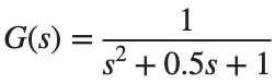
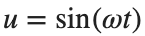
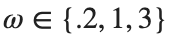
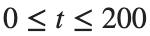
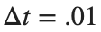
, , rad/s. s, s.
Procedure
- Calculate the output using lsim, and plot the input and output for only the final two periods.
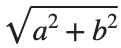
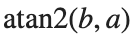
- Fit the output to by least squares to obtain gain and phase .
- Compare with the gain and phase calculated using abs and angle from the complex response of squeeze(freqresp(G,omega)). angle returns radians. Convert both phase calculations to degrees in the table.

Results to retain
- A frequency table with 3 rows and 3 plots comparing the final two periods.
s=tf('s'); G=1/(s^2+.5*s+1); omega=1; t=(0:.01:199.99)'; u=sin(omega*t);
y=lsim(G,u,t); keep=t>=t(end)-4*pi/omega;
% TODO: Fit a,b over the keep interval and calculate gain and phase.
Record results and self-check
ω [rad/s] | |
Measured gain | |
Calculated gain | |
Measured phase [deg] | |
Calculated phase [deg] |
Points to check
- Did you exclude the initial interval containing the transient?
- Did you compare errors after aligning phase units and accounting for 360° periodicity?
Comparing damping and resonance
Starting conditions
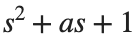
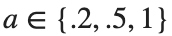
Set the denominator to and compare . Use ω=logspace(-2,2,400).
Procedure
- Plot the gains and phases of the three models on the same frequency axis.
- Tabulate each model's maximum gain, its frequency, and DC gain.
- Choose one sinusoidal condition near the maximum gain and check it using the method from the first activity.
Results to retain
- 1 set of Bode plots and a resonance comparison table.
s=tf('s'); omega=logspace(-2,2,400);
for a=[.2 .5 1]
response=squeeze(freqresp(1/(s^2+a*s+1),omega)); fprintf('a %.2g max magnitude %.9g\n',a,max(abs(response)));
end
% TODO: Complete the phase and resonance-frequency table.
Record results and self-check
a | |
Maximum gain | |
ω at maximum gain | |
DC Gain |
Points to check
- Did you distinguish dB from linear gain?
- Did you use the same frequency grid and input amplitude for all models?
Checking frequency units in the time domain
Starting conditions
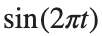
rad/s differs from Hz. The second input is .


Procedure
- First record the periods of both inputs, then calculate their responses for the same G.
- Record the phase difference both as a time delay and as an angle.
- Explain what you would misread on a Bode plot if you confused rad/s with Hz.
Results to retain
- A unit comparison table with 2 rows and output plots.
s=tf('s'); G=1/(s^2+.5*s+1);
for w=[1 2*pi], fprintf('omega %.9g, period %.9g\n',w,2*pi/w); end
% TODO: Compare the responses to the two inputs on the same time axis.
Record results and self-check
Input | |
ω [rad/s] | |
Period [s] | |
Gain | |
Phase [deg] |
Points to check
- Did you use the relationship ?
- Did you record amplitude changes and period changes as distinct phenomena?
