Frequency-Domain Stability
English translation
Execution conditions
MATLAB · Control System Toolbox
Learning objectives
Before simulating all time responses, try assessing stability from the frequency response and open-loop poles.
Unstable open-loop and closed-loop poles
Starting conditions
, ,1. Use negative unity feedback.
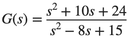

Procedure
- Count P, the number of open-loop right-half-plane poles.
- Plot the Nyquist plot for each K, and directly calculate Z, the number of closed-loop poles in the right half-plane.
- State your sign convention for the direction of encirclements of -1, and check the relationship among P, the encirclement count, and Z.
Results to retain
- 2 Nyquist plots and an assessment table.
s=tf('s'); G=(s^2+10*s+24)/(s^2-8*s+15); disp(pole(G));
for k=[.5 1], disp(k); disp(pole(feedback(k*G,1))); end
% TODO: Record the Nyquist plot and number of encirclements.
Record results and self-check
K | |
P | |
Number and direction of encirclements | |
Z | |
Closed-loop stability |
Points to check
- Did you avoid concluding that the closed loop is unstable solely because it has open-loop poles?
- Does the Nyquist assessment agree with the calculated closed-loop poles?
Stability margins and gain changes
Starting conditions
For , compare .
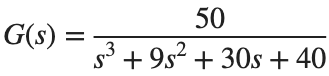
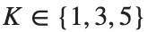
Procedure
- Find the gain margin, phase margin, and corresponding crossover frequencies using margin(K*G).
- Report gain margin separately as a linear ratio and in dB using 20log10.
- Examine each set of closed-loop poles and time response, and explain the relationship between margins and stability.
Results to retain
- A margin table and response comparison plot.
s=tf('s'); G=50/(s^3+9*s^2+30*s+40);
for k=[1 3 5]
[gm,pm,wcg,wcp]=margin(k*G); disp([k gm pm wcg wcp]);
end
% TODO: Add the gain margin columns for linear ratio and dB, along with poles and time responses.
Record results and self-check
K | |
GM [ratio] | |
GM [dB] | |
PM [deg] | |
Crossover ω [rad/s] | |
Stability |
Points to check
- Did you distinguish GM as a linear ratio from its dB value?
- Did you leave undefined or infinite margins labeled as such?
Changing the frequency range
Starting conditions
For the same G, compare examining only ω=[.1,1,10] with examining logspace(-2,3,1000).
Procedure
- Compare gain and phase on both grids.
- Describe the information missed when assessing crossover points and stability margins using only three sparse points.
- Record both calculated values and visual evidence to distinguish assessment results from plot resolution.
Results to retain
- A plot comparing resolutions and a brief interpretation.
s=tf('s'); G=50/(s^3+9*s^2+30*s+40); coarse=[.1 1 10]; fine=logspace(-2,3,1000);
% TODO: Compare the gain and phase of freqresp(G,coarse) and freqresp(G,fine).
Record results and self-check
Frequency grid | |
Observed crossover | |
Calculated GM and PM | |
Limits of the assessment |
Points to check
- Did you specify the observed frequency range and sample count?
- Did you distinguish calculated margins from visually estimated margins?