PID Control

English translation

Execution conditions

MATLAB · Control System Toolbox

Learning objectives

Selecting a gain based only on response speed can leave the system vulnerable to overshoot or model changes. Compare different performance metrics.

Baseline P, PI, and PID comparison

Starting conditions

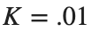
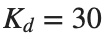
Motor parameters:

J=.01

b=.1

K=.01

R=1

L=.5

. P=(500,0,0), PI=(500,300,0), PID=(500,300,30).

Procedure

Build three closed-loop models using negative unity feedback.
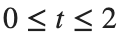
Plot the unit-step responses over $0\le t\le 2$ s in the same figure, and check the poles first.
Record overshoot, settling time, and steady-state error for stable models.

Results to retain

A table with 3 controller rows, response plots, and a brief comparison of their roles.

s=tf('s'); G=.01/((.01*s+.1)*(.5*s+1)+.01^2);
configs=[500 0 0;500 300 0;500 300 30]; names={'P','PI','PID'};
for i=1:size(configs,1)
    gains=configs(i,:); C=gains(1)+gains(2)/s+gains(3)*s; T=feedback(C*G,1);
    disp(names{i}); disp(pole(T));
end
% TODO: Record responses on the same time axis and performance metrics.
 

Record results and self-check

Controller
Kp
Ki
Kd
Stability
Overshoot [%]
Settling Time [s]
Steady-State Error

Points to check

Are the plant, input, and time axis the same, with only the controller changing?
For unstable or unconverged cases, did you give a reason instead of reporting metrics?

Changing one term at a time

Starting conditions

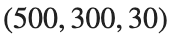
Starting from the PID baseline (500,300,30), change only Kp to 250,500,750. Keep Ki and Kd fixed.

Procedure

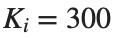
Use the PID $(500,300,30)$ result from Activity 1 as the baseline, and change only $K_p$ to 250 and 750 in turn. Keep $K_i=300$ , $K_d=30$ , the plant, and the time axis unchanged.
Plot both unit-step responses alongside the baseline curve in the same figure. Use the same stepinfo settings to calculate overshoot, settling time, and steady-state error, and record them in the same columns as Activity 1.
Choose one of the two additional settings. Use the table values to explain which metric you aim to improve over the baseline and which changes you are willing to accept.

Results to retain

Response plots and a performance table for both settings. One sentence explaining your choice.

s=tf('s'); G=.01/((.01*s+.1)*(.5*s+1)+.01^2);
for kp=[250 500 750]
    T=feedback((kp+300/s+30*s)*G,1); disp(kp); disp(dcgain(T));
end
% TODO: Compare time responses and performance metrics for the two specified Kp settings.
 

Record results and self-check

Changed term
Value
Overshoot [%]
Settling Time [s]
Steady-State Error

Points to check

Did you change only one gain at a time?
Did you support claims of faster response with specific metrics?

Input limits and integrator windup

Starting conditions

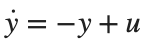
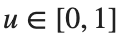
1st-order plant

\dot y=-y+u

, reference 2→.5 (changes at 5 s),

u\in[0,1]

, dt=.01 s. Use

K_p=2

K_i=1

Procedure

In the supplied PI simulation, plot the actual input alongside the input before limiting.
Compare conditional integration enabled and disabled.
Explain why the error persists after lowering the reference, relating it to the integrator state.

Results to retain

Three plots of output, input, and integrator state, and a comparison table.

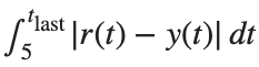
In the comparison table, IAE is

\int_{5}^{t_{\mathrm{last}}}|r(t)-y(t)|\,dt

from the reference-change time to the final recording time. Calculate input saturation duration by multiplying the number of samples where the limited u is 0 or 1 over the entire record by dt.

Use the same interval and calculation method for both integration approaches.

figure; hold on
for flag=[false true]
    [time,trace]=simulateAntiWindup(flag); plot(time,trace(:,2),'DisplayName',string(flag));
end
xlabel('Time [s]'); ylabel('Output'); legend; grid on
% TODO: Add the input, integrator state, and metrics after 5 s.
function [t,rows]=simulateAntiWindup(antiwindup)
    t=(0:.01:11.99)'; y=0; integral=0; rows=zeros(numel(t),5);
 for n=1:numel(t)
        ref=2; if t(n)>=5, ref=.5; end
        e=ref-y; raw=2*e+integral; u=min(max(raw,0),1);
 if ~antiwindup || (raw>0 && raw<1) || (raw>=1 && e<0) || (raw<=0 && e>0)
            integral=integral+e*.01;
 end
        y=y+(-y+u)*.01; rows(n,:)=[ref y raw u integral];
 end
end
 

Record results and self-check

Integration handling
IAE after the reference change
Maximum integral value
Input saturation duration [s]

Points to check

Did you distinguish input values before and after limiting?
Did you compare only integration handling without also changing the PI gains?