Reference Tracking and Optimal Control · Lesson

English translation

Execution conditions

MATLAB · Control System Toolbox

Topics covered

Examine why reference error remains even with a stable controller, and compare tracking performance with control-input cost.

Stability and reference tracking have different conditions

u=−Kx is a regulator that drives the state to the origin. For a reference r, use

u=-Kx+Nr

and calculate N from the nominal model's steady-state equation.

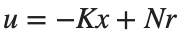
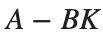
Assess stability using

A-BK

, and calculate the tracked output including the reference path.

Interpreting LQR cost

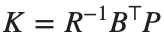
Define the cost of state deviations and input use as

J=\int(x^\top Qx+u^\top Ru)\,dt

. Increasing Q assigns a higher cost to that state deviation.

This does not mean that all metrics improve simultaneously. States with different units require normalization by reference magnitudes or interpretation of the weights' units.

This model is a 2nd-order system with normalized states and input. Under

R>0

and suitable controllability conditions, solve the CARE to obtain

K=R^{-1}B^\top P

. If the input saturates, the optimality of this linear, unconstrained design no longer applies directly.

Checking the same design in MATLAB

Reference gain adjusts the input amplitude to achieve the desired steady-state output. LQR state-feedback gain is determined by the costs assigned to state error and control input.

Same poles, different reference tracking

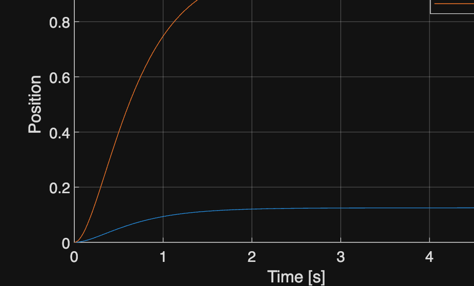
Keep the control poles fixed and change only the reference gain to examine differences in the steady-state value.

%% Worked example

A=[0 1;-2 -3]; B=[0;1]; C=[1 0]; K=place(A,B,[-2 -4]);

N=-1/(C*((A-B*K)\B)); disp(K); disp(N); assert(abs(N-8)<1e-10);

t=linspace(0,5,1001)'; figure; hold on

for gain=[1 N]

y=lsim(ss(A-B*K,B*gain,C,0),ones(size(t)),t);

     6     3

     8

plot(t,y,'DisplayName',sprintf('N=%g',gain));

end

xlabel('Time [s]'); ylabel('Position'); legend; grid on

Reference-tracking responses with the same state feedback and N=1 or N=8. Position is plotted against Time [s]; N=1 approaches a low value and N=8 approaches 1.

[Klqr,P]=lqr(A,B,diag([4 1]),1); disp(Klqr); disp(eig(A-B*Klqr));

    0.8284    0.4142

   -1.4142
   -2.0000