Root Locus · Lesson
English translation
Execution conditions
MATLAB · Control System Toolbox
Topics covered
Examine how choosing a gain relates to pole locations and the time response.
Overall workflow
Open-loop model → candidate gains → closed-loop poles → time response
Paths of poles as gain changes
The closed-loop poles with unity feedback are the roots of 1+K L(s)=0. The root locus shows how these roots move as K changes.
When choosing a K, examine all poles corresponding to that K together.
Checking pole choices through responses
If any pole has a positive real part, stable step-response metrics cannot be calculated. Even for stable candidates, zeros, residues, and inputs affect the response. Compare damping and speed predicted from poles with the actual curves before selecting a gain.
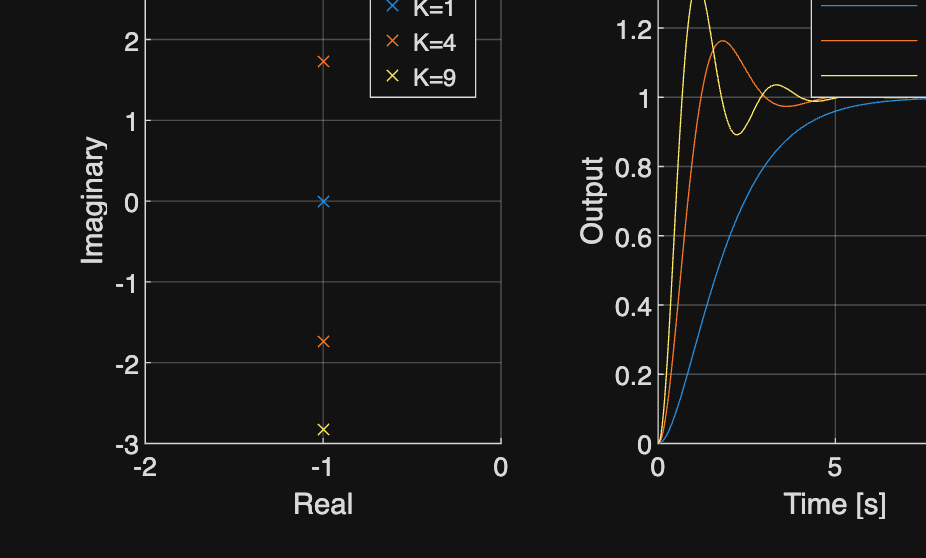
Closed-loop poles that change with gain
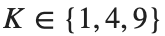
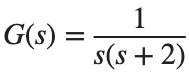
Apply to . Examine the pole map and step response together.
%% Worked example
s=tf('s'); G=1/(s*(s+2)); t=linspace(0,10,1001)';
figure; tiledlayout(1,2); ax1=nexttile; hold(ax1,'on'); ax2=nexttile; hold(ax2,'on');
for gain=[1 4 9]
T=feedback(gain*G,1); p=pole(T); [y,tm]=step(T,t);
plot(ax1,real(p),imag(p),'x','DisplayName',sprintf('K=%g',gain));
plot(ax2,tm,y,'DisplayName',sprintf('K=%g',gain));
end
xlabel(ax1,'Real'); ylabel(ax1,'Imaginary'); xlabel(ax2,'Time [s]'); ylabel(ax2,'Output');
grid(ax1,'on'); grid(ax2,'on'); legend(ax1); legend(ax2);
Reference example
View more examples