System Modeling

English translation

Execution conditions

MATLAB · Control System Toolbox

Place the measurement file step_measurements.csv in the same folder as the script. The code downloads it if it is missing.

To obtain positive gain and time constant, estimate their logarithms using fminsearch.

Learning objectives

Use the model to determine whether changing mass or resistance affects the transient response, the steady-state value, or both.

Cruise model and units

Starting conditions

m=1000

kg,

b=50

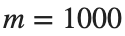
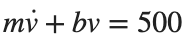
N·s/m, force 500 N. The state and output are velocity [m/s].

Procedure

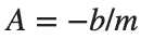
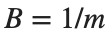
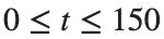
Build a model using $A=-b/m$ , $B=1/m$ , $C=1$ , and $D=0$ , and plot the response over $0\le t\le150$ s to a constant force of 500 N.
Change only $m\in\{500,1000,1500\}$ and apply the same force. Substitute $\dot v=0$ into $m\dot v+bv=500$ to obtain steady-state velocity, and match the coefficients of $\dot v+(b/m)v=500/m$ to the standard 1st-order form to obtain the time constant.
For each mass, record the calculated steady-state velocity alongside the final simulation sample $v(150)$ . Find when the curve reaches approximately 63.2% of the calculated steady-state velocity, and compare this time with the calculated time constant.

Results to retain

A table of 3 mass conditions, 1 velocity plot, and a brief explanation of the properties changed by mass.

m=1000; b=50; force=500;
G=ss(-b/m,1/m,1,0); t=linspace(0,150,1501)';
[v,tm]=step(force*G,t); figure; plot(tm,v);
xlabel('Time [s]'); ylabel('Linear Velocity [m/s]'); grid on
% TODO: Compare numerical results for the three mass conditions with the values predicted by the equations.
 

Record results and self-check

m [kg]
Predicted final velocity [m/s]
Measured velocity [m/s]
Time Constant [s]

Points to check

Did you avoid multiplying by the input force 500 twice?
For fixed b, does changing mass affect the time constant rather than the steady-state velocity?

Comparing motor-model coefficients

Starting conditions

J=.01

b=.1

K=.01

L=.5

. Compare

R\in\{.5,1,2\}

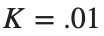
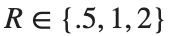
Ω with an input of 1 V.

Procedure

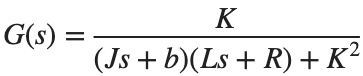
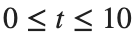
Construct $G(s)=\frac K{(Js+b)(Ls+R)+K^2}$ and calculate its response over $0\le t\le 10$ s.
Tabulate the poles, DC gain, and final output for each R.
Explain which terms in the equation change with electrical resistance and inertia.

Results to retain

3 response curves and 1 coefficient table.

s=tf('s'); J=.01; b=.1; K=.01; L=.5;
for R=[.5 1 2]
    G=K/((J*s+b)*(L*s+R)+K^2); disp(R); disp(pole(G)); disp(dcgain(G));
end
% TODO: Add the three responses on the same time axis.
 

Record results and self-check

R [Ω]
Pole
DC Gain
Final velocity [rad/s]

Points to check

Did you use the same J, b, K, L, and input for all conditions?
Did you compare the long-term output with 1 V×DC gain?

Estimating a model from a measured response

Starting conditions

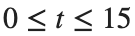
Synthetic sensor step record:

y=1.8(1-e^{-t/3})+\text{noise}

0\le t\le 15

s, 151 points, noise standard deviation .03, seed=7.

Procedure

Read the supplied step_measurements.csv and estimate $K,\tau$ using fminsearch in the starter code. Keep the code that optimizes the logarithms of the estimated variables.
Apply the same estimation separately to the full 0–15 s record and the first 0–3 s. Tabulate the sample count and estimated $K,\tau$ for each interval.
Plot each fitted curve on the same time axis as the measurements, and plot residuals as measured minus estimated values. Based on the final values and residual patterns, choose one time interval where you would like more measurements and explain why.

Results to retain

A table of estimates for both measurement intervals and response and residual plots.

dataFile=fullfile(fileparts(mfilename('fullpath')),'step_measurements.csv');
if ~isfile(dataFile)
    websave(dataFile,'https://nii-lab.github.io/assets/courses/control-2/system-modeling/step_measurements.csv');
end
data=readmatrix(dataFile); tm=data(:,1); measured=data(:,2);
response=@(time,par) par(1)*(1-exp(-time/par(2)));
for finish=[3 15]
    select=tm<=finish;
    loss=@(logpar) sum((response(tm(select),exp(logpar))-measured(select)).^2);
    logpar=fminsearch(loss,log([1 2]),optimset('Display','off','TolX',1e-10,'TolFun',1e-12));
    parameters=exp(logpar); disp(finish); disp(parameters);
end
% TODO: Plot responses and residuals to compare results from the two measurement intervals.
 

Record results and self-check

Recording interval [s]
Estimated gain
Estimated time constant [s]
RMSE

Points to check

Did you estimate the synthetic data as if their generating settings were unknown, as with actual measurements?
Did you avoid assessing uncertainty from a short record using residual size alone?

Official examples and data

SciPy · curve_fit