Transfer Function · Lesson

English translation

Execution conditions

MATLAB · Control System Toolbox

Topics covered

Even with the same coefficients, responses depend on the interconnection and cancellation conditions. Practice predicting behavior from coefficients.

Overall workflow

Coefficient arrays → transfer function → poles and zeros → step response

Interpreting coefficient arrays as transfer functions

Coefficient arrays: highest power first.
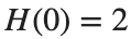
num=[2], den=[5,1]: $H(s)=2/(5s+1)$ .
Poles: roots of the denominator. In this example, $-0.2$ .
Zeros: roots of the numerator. This example has no finite zeros.
DC gain: $H(0)=2$ . The denominator's constant term is not 0.

Connecting poles to actual responses

The time constant of exp(−0.2t), corresponding to the negative real pole −0.2, is 5 s. Examining the roots calculated from coefficients alongside the time response reveals the physical meaning of the calculation.

Series connection multiplies, parallel connection adds, and negative unity feedback also changes the denominator, giving H/(1+H).

Cancellation of common factors

(s+2)/((s+1)(s+2)) can be expressed as 1/(s+1) after cancellation. If the numerator's 2 changes to 2.1, cancellation is no longer exact. Examine both the model order and small response differences.

From coefficients to poles and responses

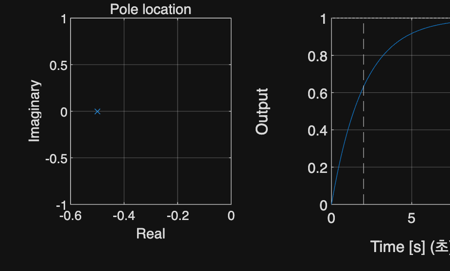
H(s)=1/(2s+1) has a pole at −0.5, a DC gain of 1, and a time constant of 2 s. Examine the equation and plot together below.

%% Worked example

s=tf('s'); H=1/(2*s+1); t=linspace(0,10,501)';

disp('Pole / Zero / DC Gain'); disp(pole(H)); disp(zero(H)); disp(dcgain(H));

Pole / Zero / DC Gain
   -0.5000

     1

figure; tiledlayout(1,2);

nexttile; plot(-.5,0,'x'); xline(0); xlabel('Real'); ylabel('Imaginary'); title('Pole location'); grid on

nexttile; step(H,t); xline(2,'--'); xlabel('Time [s]'); ylabel('Output'); title('Unit step'); grid on

Pole location and unit-step response of H(s)=1/(2s+1). Left: a cross at (-0.5,0). Right: Output rises from 0 toward 1 against Time [s], with a vertical dashed line at t=2 s.

Reference example

View more examples

Reference materials