Compensator Design · Lesson

English translation

Execution conditions

MATLAB · Control System Toolbox

Topics covered

Decide whether to adjust lead or lag compensation when speed, damping, and steady-state error must be met together.

Overall workflow

Performance targets → compensator poles and zeros → closed-loop response → compare speed and error

Defining the compensator's role

Add poles and zeros when a single gain cannot meet response-speed, damping, and steady-state-error targets together. First define the desired performance numerically with units, then choose a compensator type.

Distinguishing design from validation

Lead compensation mainly adjusts phase and speed; lag compensation mainly adjusts low-frequency gain and steady-state error. Even if the design point is met, input cost or other poles may cause problems.

Examine the compensated and uncompensated responses using the same step and ramp conditions and sufficiently long recording intervals.

Lead compensation with the same DC gain

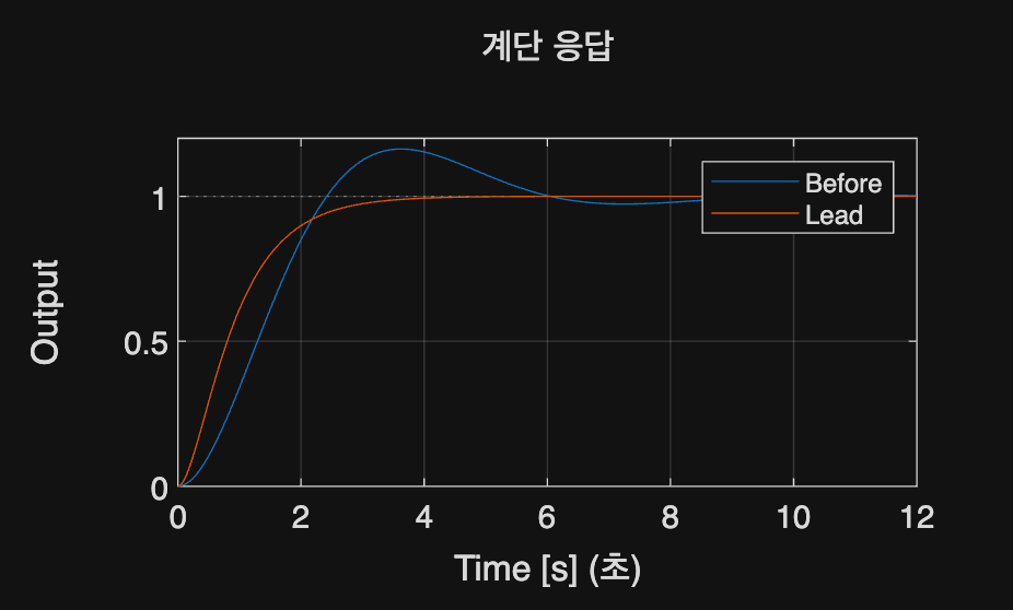
Compare G(s)=1/(s(s+1)) and C(s)=(s+1)/(0.2s+1). Examine how the response shape changes while keeping C's DC gain at 1.

%% Worked example

s=tf('s'); G=1/(s*(s+1)); C=(s+1)/(.2*s+1); t=linspace(0,12,1201)';

figure; step(feedback(G,1),feedback(C*G,1),t); legend('Before','Lead');

xlabel('Time [s]'); ylabel('Output'); grid on; disp(dcgain(C));

Step responses before and after lead compensation. Output is plotted against Time [s]; Before rises above 1 before approaching 1, while Lead rises toward 1.

1

Reference example

View more examples

Reference materials