Frequency-Domain Stability · Lesson

English translation

Execution conditions

MATLAB · Control System Toolbox

Topics covered

Before simulating all time responses, try assessing stability from the frequency response and open-loop poles.

Overall workflow

Open-loop poles → Nyquist plot → stability margins → check closed-loop poles

Nyquist and open-loop poles

Counting only encirclements of −1 can lead to an incorrect stability assessment. Use both the number of open-loop right-half-plane poles and the sign of the encirclement direction, and check against directly calculated closed-loop poles.

Conditions for interpreting stability margins

The gain crossover frequency is where the open-loop response magnitude is 1. The difference between the phase at this frequency and −180° is the phase margin.

At a frequency where phase is −180°, the reciprocal of the response magnitude is the gain margin. Mark crossover points on the Bode plot to show where both margins are calculated.

Checking frequency response and closed-loop poles

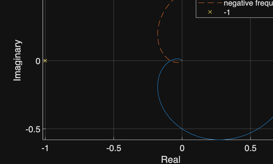
Examine the Nyquist plot and closed-loop poles of L(s)=5/((s+1)(s+2)(s+3)). This example has no open-loop right-half-plane poles.

%% Worked example

s=tf('s'); L=5/((s+1)*(s+2)*(s+3)); omega=logspace(-3,3,1000);

z=squeeze(freqresp(L,omega)); figure;

plot(real(z),imag(z),real(z),-imag(z),'--'); hold on; plot(-1,0,'x');

xlabel('Real'); ylabel('Imaginary'); axis equal; grid on

legend('positive frequency','negative frequency','-1'); disp(pole(feedback(L,1)));

Complex-plane frequency response of L(s)=5/((s+1)(s+2)(s+3)). Axes are Real and Imaginary. Solid positive-frequency and dashed negative-frequency curves are mirrored across the real axis; a cross marks (-1,0).

  -3.9042 + 0.0000i
  -1.0479 + 1.3112i
  -1.0479 - 1.3112i

Reference example

View more examples

Reference materials