Laplace Transform · Lesson

English translation

Execution conditions

MATLAB: Symbolic Math Toolbox required.

If ver('symbolic') returns an empty result, install Symbolic Math Toolbox from MATLAB Add-Ons.

Topics covered

Directly verify that the solution obtained by transforming a time-domain differential equation satisfies the original problem.

Overall workflow

Differential equation and initial values → s-domain equation → Y(s) → time response and residuals

Examining expressions and their domains

Canceling common factors in a rational expression simplifies calculations. However, values that make the original denominator 0 must still be excluded. For example,

\frac{x-1}{x-1}

equals 1 at

x\ne1

, but at

x=1

the original expression is undefined.

Converting a differential equation to an algebraic equation

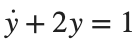
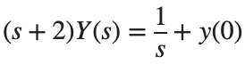
Applying the Laplace transform to

\dot y+2y=1

separates the effects of input and initial state into distinct terms.

(s+2)Y(s)=\frac{1}{s}+y(0)

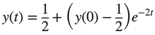
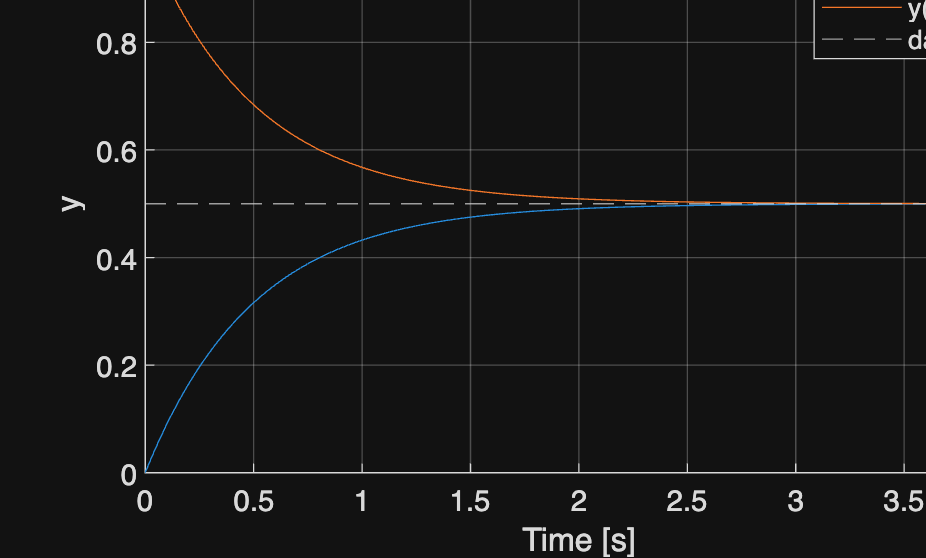
The two solutions for different initial values are shown below.

y(t)=\frac12+\left(y(0)-\frac12\right)e^{-2t}

Substituting y(0)=0 and 1 gives the same steady-state value but different starting points and transient responses.

Two responses with different initial values

For

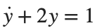
\dot y+2y=1

, compare y(0)=0 and 1. Plot both solutions on the same time axis and check their initial and steady-state values.

%% Worked example

t=linspace(0,4,401)';

figure; hold on

for initialValue=[0 1]

y=.5+(initialValue-.5)*exp(-2*t);

plot(t,y,'DisplayName',sprintf('y(0)=%g',initialValue));

end

yline(.5,'--'); xlabel('Time [s]'); ylabel('y'); legend; grid on

Responses with initial values y(0)=0 and y(0)=1 against Time [s]. One rises from 0 and the other falls from 1; both approach the dashed y=0.5 line.

Reference example

View more examples

Reference materials