Laplace Transform

English translation

Execution conditions

MATLAB: Symbolic Math Toolbox required.

If ver('symbolic') returns an empty result, install Symbolic Math Toolbox from MATLAB Add-Ons.

Learning objectives

Directly verify that the solution obtained by transforming a time-domain differential equation satisfies the original problem.

Checking that simplification preserves values

Starting conditions

D=\frac{x^2-2x+1}{x^2-3x+2}

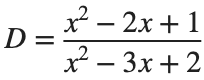
: simplify by cancellation. For value comparisons, use

x\in\{0,3\}

Procedure

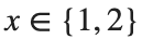
Simplify D by cancellation, and separately identify the x values that make the original denominator 0.
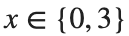
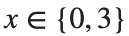
At $x\in\{0,3\}$ , check that the values before and after cancellation agree. Explain why $x\in\{1,2\}$ cannot be checked in the same way.

Results to retain

Expressions before and after cancellation, excluded values, and substitution results at the two points.

assert(exist('sym','file')~=0,'Symbolic Math Toolbox is required.');
syms x
D=(x^2-2*x+1)/(x^2-3*x+2);
disp('약분한 식'); disp(simplify(D)); disp('원래 분모의 근'); disp(solve(x^2-3*x+2==0,x));
% TODO: Compare values at x=0,3 and explain the two points to exclude.
 

Record results and self-check

Original expression before cancellation
Expression after cancellation
Excluded x values
Value difference at the two points

Points to check

Did you identify both values that make the original denominator 0?
Did you avoid substituting $x=1$ into the original expression based only on its simplified form?

Laplace transform and inverse transform

Starting conditions

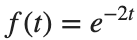
For t>0, transform

f(t)=e^{-2t}

, then take its inverse transform.

Procedure

Use laplace and ilaplace to obtain the transform and inverse transform.
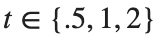
Compare the original and recovered function values at $t\in\{.5,1,2\}$ .
Explain how the pole −2 of the transformed expression relates to the time-domain decay term $e^{-2t}$ .

Results to retain

A short table of F(s), the recovered function, and numerical differences.

syms t positive
syms s
f=exp(-2*t); F=laplace(f,t,s); restored=ilaplace(F,s,t);
disp(F); disp(restored);
% TODO: Find the differences between the original function and inverse transform at the three specified times.
 

Record results and self-check

Function
F(s)
Inverse transform
Maximum numerical error

Points to check

Did you record the positive assumption for t and the initial condition?
At the same t>0, is the numerical error between the original function and its inverse transform at most 1e-8?

Differential equations with initial conditions

Starting conditions

\dot y+2y=1

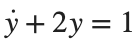
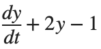
; compare y(0)=0 with y(0)=1. The input is a unit step for t≥0.

Procedure

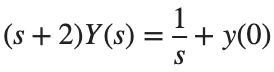
Write the Laplace transform of the derivative term and substitute the initial condition to obtain $(s+2)Y(s)=\frac1s+y(0)$ .
Divide both sides of this equation by $s+2$ to obtain $Y(s)$ . Substitute each initial condition, take the inverse transform, and plot both $y(t)$ over $0\le t\le4$ s together.
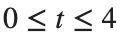
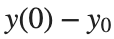
For each $y(t)$ , calculate $\frac{dy}{dt}+2y-1$ and $y(0)-y_0$ . Record both residuals for each initial condition and determine whether they are 0.

Results to retain

Two response curves, a residual table, and a brief explanation of the initial condition's role.

syms t positive
syms s
for y0=[0 1]
    Y=(1/s+y0)/(s+2); y=ilaplace(Y,s,t); disp(y0); disp(y);
end
% TODO: Add initial-condition and ODE residuals, and both response plots.
 

Record results and self-check

y(0)
Y(s)
Initial-value residual
ODE residual
Steady-state value

Points to check

Did the input and initial condition enter as separate terms?
Is the symbolic residual 0, and do both responses have the same steady-state value?