Model Uncertainty and Robustness · Lesson

English translation

Execution conditions

MATLAB · Control System Toolbox

Topics covered

Apply a controller designed for one model to several actual models and delay conditions to find where performance deteriorates.

Nominal and actual models

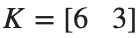
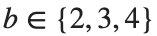
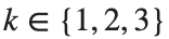
The plant is

m\ddot y+b\dot y+ky=u

, with state-feedback gain fixed at

K=\left[\begin{array}{cc}6&3\end{array}\right]

. Using all combinations of mass

m\in\{0.7,1,1.3\}

, damping

b\in\{2,3,4\}

, and stiffness

k\in\{1,2,3\}

gives

3^3=27

models to check.

Examining stability and performance separately

Assess stability from each model's poles, and compare steady-state error and settling time in the step responses. The performance table for the 27 combinations reports results at the selected values.

Before applying input delay and saturation, stability of the linear model can be assessed using the characteristic polynomial

ms^2+(b+3)s+(k+6)

. If all three coefficients of a 2nd-order polynomial are positive, its poles have negative real parts. All three coefficients are positive throughout the given

m,b,k

range, so the system is stable throughout that range.

Response speed and error depend on the parameters.

Checking the same design in MATLAB

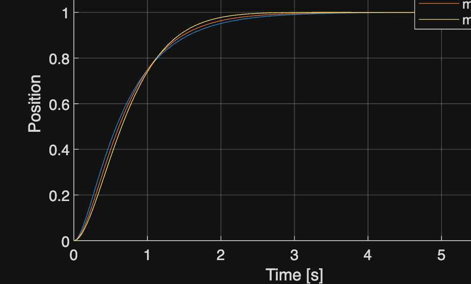
Keep the designed gain fixed and change only the plant's mass, damping, and stiffness. The poles of each combination indicate stability; the response curves show changes in overshoot and settling time.

Actual systems with different masses

Keep the same controller and change only mass to compare poles and time responses.

%% Worked example

A0=[0 1;-2 -3]; B0=[0;1]; C=[1 0]; K=place(A0,B0,[-2 -4]); N=8;

t=linspace(0,6,1201)'; figure; hold on

for m=[.7 1 1.3]

A=[0 1;-2/m -3/m]; B=[0;1/m]; p=eig(A-B*K);

y=lsim(ss(A-B*K,B*N,C,0),ones(size(t)),t);

fprintf('mass %.2f\n',m); disp(p); plot(t,y,'DisplayName',sprintf('m=%g',m));

mass 0.70
   -1.6516
   -6.9199

mass 1.00
    -2
    -4

mass 1.30
  -2.3077 + 0.9102i
  -2.3077 - 0.9102i

end

xlabel('Time [s]'); ylabel('Position'); legend; grid on

Position responses for m=0.7, 1 and 1.3 against Time [s]. The three curves differ slightly during their rise and approach values near 1.

Official documentation and data

SciPy · Pole placement