Model Uncertainty and Robustness

English translation

Execution conditions

MATLAB · Control System Toolbox

Learning objectives

Apply a controller designed for one model to several actual models and delay conditions to find where performance deteriorates.

Applying the nominal controller to other actual models

Starting conditions

m\in\{.7,1,1.3\}

kg,

b=3

N·s/m,

k=2

N/m. Fix K and N at the values designed for

m=1

Procedure

Keep the nominal controller fixed and compare the poles and responses of the three actual models.
Find the final value and 2% settling time of each response, and identify the slowest condition.

Results to retain

Three response curves and a comparison table of poles and settling times.

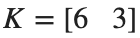
A0=[0 1;-2 -3]; B0=[0;1]; C=[1 0]; K=place(A0,B0,[-2 -4]); N=8;
t=linspace(0,6,1201)'; figure; hold on
for m=[.7 1 1.3]
    A=[0 1;-2/m -3/m]; B=[0;1/m]; p=eig(A-B*K);
    y=lsim(ss(A-B*K,B*N,C,0),ones(size(t)),t);
    fprintf('mass %.2f\n',m); disp(p); plot(t,y,'DisplayName',sprintf('m=%g',m));
end
xlabel('Time [s]'); ylabel('Position'); legend; grid on
 

Record results and self-check

Mass
Pole
Final value
Settling Time

Points to check

Did you keep K unchanged rather than redesigning it for each actual model?
Did you check that the response stays within the 2% band after the settling time?

Changing mass, friction, and stiffness together

Starting conditions

Use the 27 combinations of m∈{.7,1,1.3}, b∈{2,3,4}, and k∈{1,2,3}. Keep

K=\left[\begin{array}{cc}6&3\end{array}\right]

and

N=8

fixed.

Procedure

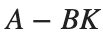
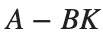
For each combination, find the maximum real part of the eigenvalues of $A-BK$ . Record the number of models where this value is negative and where it is 0 or greater.
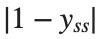
Find the combination with the largest maximum real part. Also calculate $y_{ss}=-C(A-BK)^{-1}BN$ for each combination, and separately find the combination with the largest $|1-y_{ss}|$ .
For the two selected combinations, tabulate $m,b,k$ , maximum pole real part, and steady-state error, and plot unit-step responses on the same time axis.
Distinguish the parameter values checked in this calculation from the unchecked values between them. Explain which coefficient conditions in the learning material's characteristic polynomial should be examined to assess stability over the entire range.

Results to retain

A stability summary for the 27 conditions and responses for the two extreme cases.

records=[];
for m=[.7 1 1.3]
 for b=[2 3 4]
 for k=[1 2 3]
    A=[0 1;-k/m -b/m]; B=[0;1/m]; aa=A-B*K;
    maxReal=max(real(eig(aa))); final=-C*(aa\(B*N)); records(end+1,:)=[m b k maxReal abs(1-final)];
 end
 end
end
[~,near]=max(records(:,4)); [~,large]=max(records(:,5)); disp(records(near,:)); disp(records(large,:));
% TODO: Add the unit-step responses of these two models on the same time axis.
 

Record results and self-check

m,b,k
Maximum pole real part
Steady-State Error

Points to check

Did you calculate poles from $A-BK$ rather than A?
Did you distinguish pole calculations for the 27 combinations from analytical justification covering the entire parameter range?

With input delay and saturation

Starting conditions

Euler-integrate the nominal model's state with dt=.002 s steps for 6 s. Input delays are 0,.08,.2 s, and the input limit is ±4.

Procedure

Use the practice notebook's function to plot outputs and inputs for the three delays.
Halve dt and check that the main responses remain similar.
Explain why linear-pole stability alone is insufficient to assess an implementation with delay and saturation.

Results to retain

Output and input curves, RMS tracking error (after 2 s), input saturation fraction (the full 0–6 s record), and comparison of integration time steps.

figure; hold on
for delay=[0 .08 .2]
    [tt,yy,uu]=delayedInput(delay,.002,A0,B0,K,N); keep=tt>=2;
    disp([delay sqrt(mean((1-yy(keep)).^2)) mean(abs(uu)>=4-1e-8)]);
    plot(tt,yy,'DisplayName',sprintf('delay=%g',delay));
end
xlabel('Time [s]'); ylabel('Position'); legend; grid on
% TODO: Compare the input plots and dt=.001 results.
function [times,ys,us]=delayedInput(delay,dt,A0,B0,K,N)
    times=(0:dt:6)'; x=zeros(2,1); commands=zeros(size(times)); ys=zeros(size(times)); us=zeros(size(times)); lag=round(delay/dt);
 for n=1:numel(times)
        command=min(max(N-K*x,-4),4); commands(n)=command;
 if n>lag, u=commands(n-lag); else, u=0; end
        ys(n)=x(1); us(n)=u; x=x+dt*(A0*x+B0*u);
 end
end
 

Record results and self-check

Delay
dt
RMS tracking error
Input saturation fraction

Points to check

Is delay implemented by retrieving past inputs from the command history?
Did you avoid confusing time-step effects with model instability?

Official examples and data

SciPy · Pole placement