
State Feedback and Observer
English translation
Execution conditions
MATLAB · Control System Toolbox
Learning objectives
Estimate velocity to control a system that measures only position, and compare estimated velocity and noise sensitivity.
Can measurements distinguish states?
Starting conditions
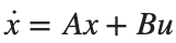
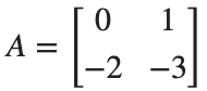
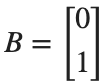
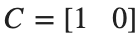
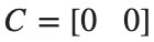
With position [m] and velocity [m/s] as states, use , . Use , , .

Procedure
- Form the controllability matrix [B,AB] and observability matrix [C;CA], and find their ranks.
- Compare the case where B is a zero vector with the case .
- Explain the distinction between an ineffective input and an unavailable measurement.
Results to retain
- A comparison table of both ranks and feasible designs for the three conditions.
A=[0 1;-2 -3]; B=[0;1]; C=[1 0];
cases={{B,C},{zeros(size(B)),C},{B,zeros(size(C))}}; names={'base','no input','no sensor'};
for i=1:numel(cases)
inputs=cases{i}; b=inputs{1}; c=inputs{2};
fprintf('%s: Controllability rank %d, Observability rank %d\n',names{i},rank(ctrb(A,b)),rank(obsv(A,c)));
end
% TODO: State the feasible control and estimation designs under each condition.
Record results and self-check
Condition | |
Controllability rank | |
Observability rank | |
Design feasibility |
Points to check
- Are both ranks of the baseline model 2?
- Did you avoid applying pole placement directly to a rank-deficient model?
Connecting state feedback and observer
Starting conditions
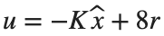
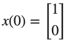
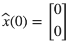
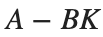
, . Control poles: −2,−4; observer poles: −8,−10. Use , .

Procedure
- Calculate K and L, and compare the eigenvalues of and .
- Integrate actual and estimated states simultaneously, and plot position, velocity, and estimation errors over 0–4 s.
- Distinguish the reduction in estimation error from the output approaching its reference.

Results to retain
- Two plots of actual and estimated position and actual and estimated velocity, and the final estimation errors.
K=place(A,B,[-2 -4]); L=place(A',C',[-8 -10])';
a_aug=[A -B*K;L*C A-B*K-L*C]; b_aug=[8*B;8*B]; t=linspace(0,4,801)';
z=lsim(ss(a_aug,b_aug,eye(4),zeros(4,1)),ones(size(t)),t,[1;0;0;0]);
figure; tiledlayout(2,1);
nexttile; plot(t,z(:,1),t,z(:,3),'--'); ylabel('Position [m]'); legend('state','estimate'); grid on
nexttile; plot(t,z(:,2),t,z(:,4),'--'); ylabel('Linear Velocity [m/s]'); xlabel('Time [s]'); legend('state','estimate'); grid on
disp(norm(z(end,1:2)-z(end,3:4)));
% TODO: Print and compare the controller and observer poles separately.
Record results and self-check
K | |
L | |
Control poles | |
Observer Pole | |
Final error |
Points to check
- Do the eigenvalues of and , after substituting the calculated K and L, match the specified control and observer poles, respectively?
- At s, are the position and velocity estimation errors below 1e-6 m and 1e-6 m/s, respectively?


Is a faster observer always better?
Starting conditions
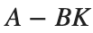
Add n(t)=0.02*sin(40*t) to the measurement. Compare observer poles (−8,−10) and (−20,−25), keeping controller K fixed.
Procedure
- Use both observer settings in the practice notebook's function, and compare the control input u on the same time axis.
- Calculate position-error RMS, velocity-error RMS, and control-input RMS separately after 1 s.
- Interpret initial estimation-error convergence separately from the response to measurement noise.
Results to retain
- Control-input curves, a comparison table of the three RMS values, and justification for the selected setting.
figure; hold on
for poles={[-8 -10],[-20 -25]}
[u,err,rms_u]=noisyObserver(poles{1},A,B,C,K,t);
plot(t,u,'DisplayName',mat2str(poles{1})); disp(poles{1}); disp(err); disp(rms_u);
end
xlabel('Time [s]'); ylabel('u [N]'); legend; grid on
% TODO: Choose an observer setting based on the metrics and explain why.
function [u,err,rms_u]=noisyObserver(poles,A,B,C,K,t)
L=place(A',C',poles)'; aa=[A -B*K;L*C A-B*K-L*C];
bb=[8*B zeros(2,1);8*B L]; inputs=[ones(size(t)) .02*sin(40*t)];
z=lsim(ss(aa,bb,eye(4),zeros(4,2)),inputs,t,[1;0;0;0]);
u=8-z(:,3:4)*K'; keep=t>=1;
err=sqrt(mean((z(keep,1:2)-z(keep,3:4)).^2,1)); rms_u=sqrt(mean(u(keep).^2));
end
Record results and self-check
Observer Pole | |
Position error RMS [m] | |
Velocity error RMS [m/s] | |
Input RMS [N] | |
Reason for your choice |
Points to check
- Are noise, initial conditions, and time steps the same for both settings?
- Did you avoid conflating error and input in a single metric?