System Modeling · Lesson

English translation

Execution conditions

MATLAB · Control System Toolbox

Place the measurement file step_measurements.csv in the same folder as the script. The code downloads it if it is missing.

To obtain positive gain and time constant, estimate their logarithms using fminsearch.

Topics covered

Use the model to determine whether changing mass or resistance affects the transient response, the steady-state value, or both.

Overall workflow

Physical equations and units → state-space model → measured response → coefficient estimation and residuals

Choosing inputs and states from physical equations

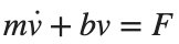
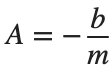
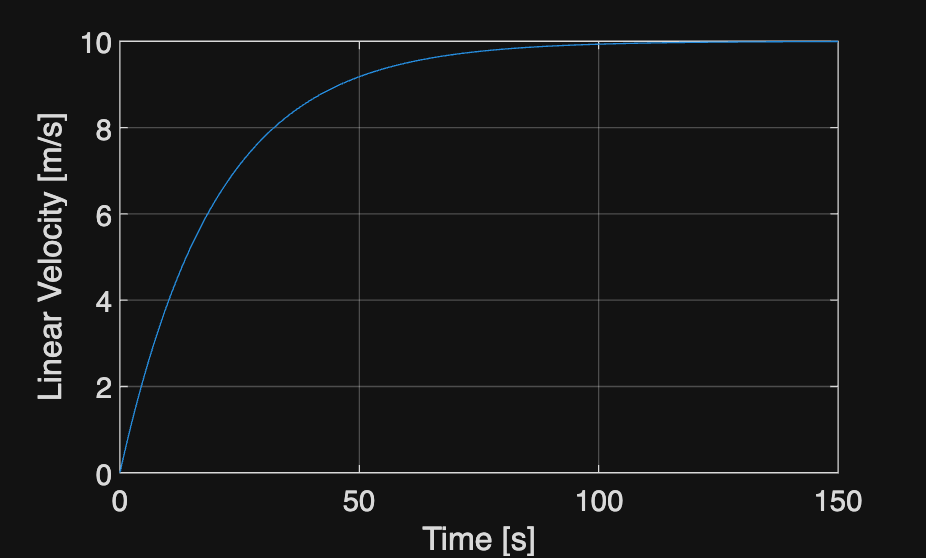
In the cruise model

m\dot v+bv=F

, the input is force, and the state and output are velocity.

A=-\frac bm

B=\frac1m

. For constant force, the final velocity is

\frac Fb

and the time constant is

\frac mb

Increasing mass leaves the final velocity unchanged but makes the velocity change more slowly.

Checking the model against measurements

In the unit-step response

y(t)=K(1-e^{-t/\tau})

, K is the steady-state value, and τ is the time to reach approximately 63.2% of that value. Fit this equation to the measured response to estimate both parameters.

The first 3 s of this example capture only the rising response. Compare how much the estimated final value and time constant change when the 15 s record is also used.

Worked example

m=1000

kg,

b=50

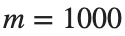
N·s/m, force 500 N. The state and output are velocity [m/s].

%% Worked example

m=1000; b=50; force=500;

G=ss(-b/m,1/m,1,0); t=linspace(0,150,1501)';

[v,tm]=step(force*G,t); figure; plot(tm,v);

xlabel('Time [s]'); ylabel('Linear Velocity [m/s]'); grid on

Linear velocity response to a constant force of 500 for the model with m=1000 and b=50. Over Time [s] from 0 to 150, velocity rises from 0 toward about 10 m/s and levels off.

Official documentation and data

SciPy · curve_fit

Reference example

View more examples

Reference materials