Transfer Function
English translation
Execution conditions
MATLAB · Control System Toolbox
Learning objectives
Even with the same coefficients, responses depend on the interconnection and cancellation conditions. Practice predicting behavior from coefficients.
From coefficients to poles and zeros
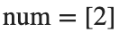
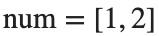
- num: coefficient array of the numerator polynomial.
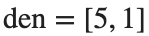
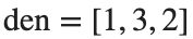
- den: coefficient array of the denominator polynomial.
- Array order: highest power first.
Starting conditions
- A: , .
- B: , .
- C: , .
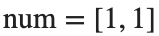
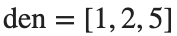
Procedure
- Run A as the baseline example. Write the numerator and denominator as polynomials, and calculate using roots and pole/zero.
- Apply the same procedure to B and C. Distinguish numerator and denominator degrees from the number of finite zeros, and record both real and imaginary parts of complex roots.
- Plot the poles and zeros of all three models on one complex plane. Use × for poles and ○ for zeros, with a different color for each model.
Results to retain
- 1 table with one row per model and 1 pole–zero map.
- Example level for A: H(s)=2/(5s+1), pole -0.2, no finite zeros. Complete B and C yourself.
- Briefly explain the relationship between coefficients and roots.
s=tf('s');
models={tf(2,[5 1]),tf([1 2],[1 3 2]),tf([1 1],[1 2 5])};
H_A=models{1}; disp(H_A); disp(pole(H_A)); disp(zero(H_A)); disp(dcgain(H_A));
% TODO: Complete the tables and complex-plane plots for B, C.
Record results and self-check
Model | |
H(s) | |
Pole | |
Finite zeros | |
DC Gain |
Points to check
- Do the roots calculated directly from the coefficients match the library results, apart from their order?
- When the denominator's constant term is not 0, does DC gain equal the ratio of constant terms?
Comparing series, parallel, and feedback connections
Starting conditions
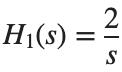
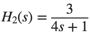
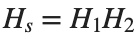
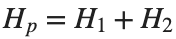
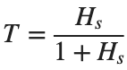
, . Use negative unity feedback for .

Procedure
- Derive expressions for , , and .
- Use series, parallel, feedback to build the same models, and compare with the directly derived expressions at ω=[0.1,1,10] rad/s.
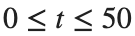
- Plot the unit-step response of T over s. Distinguish the poles at the origin of Hs and Hp from the meaning of DC gain.
Results to retain
- 1 coefficient table for the 3 interconnections and 1 step plot of T.
- Record the error as the absolute difference between complex responses at the same frequency.
s=tf('s'); H1=tf(2,[1 0]); H2=tf(3,[4 1]);
Hs=series(H1,H2); Hp=parallel(H1,H2); T=feedback(Hs,1); disp(Hs); disp(Hp); disp(T);
t=linspace(0,50,2501)'; figure; step(T,t); xlabel('Time [s]'); ylabel('Output'); grid on
% TODO: Compare with the directly derived transfer functions at the same frequencies.
Record results and self-check
Interconnection | |
Derived numerator | |
Derived denominator | |
Maximum frequency-response error |
Points to check
- Is the response difference between the two representations at most 1e-6? Did you divide all coefficients by the same value to normalize the denominator's leading coefficient to 1 before comparing?
- Does the step plot show time [s], output, and a sufficiently long recording interval?
Cancellation and small coefficient changes
Starting conditions
Create model D by changing B's numerator from [1,2] to [1,2.1]. Both models have denominator [1,3,2].
Procedure
- Record the original pole–zero maps of B and D alongside the models simplified with minreal.
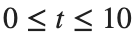
- Plot the difference between the two responses to the same unit-step input over s.
- Distinguish exact from near cancellation, and explain why the model before cancellation should also be retained.
Results to retain
- 1 model-order table and a response-difference plot.
- A brief explanation of the tolerance used to identify cancellation and its interpretation.
B=tf([1 2],[1 3 2]); D=tf([1 2.1],[1 3 2]); disp(minreal(B)); disp(minreal(D));
% TODO: Plot the unit-step responses of B, D and their difference on the same time axis.
Record results and self-check
Model | |
Original order | |
Order after simplification | |
Maximum response difference |
Points to check
- Did you avoid assuming that D has the same canceled model as B?
- Did you distinguish model representation order from actual response differences?