Control Engineering I · Week 09 · Closed-loop Gain and Sensitivity

English translation

Edit the code and response fields in your own copy. Name: ⟦enter here⟧ / Student ID: ⟦enter here⟧

How to run

In Live Editor, click inside the code and run the current section with Run Section (Windows/Linux Ctrl+Enter, Mac ⌘+Enter). Run executes the entire document. Edit the explanations and response fields directly.

Initially run from the top, and rerun any section whose values you change. If an undefined-variable error occurs, run the preceding sections first. Outputs appear below or to the right of the code.

Environment: MATLAB Online and Control System Toolbox.

1. Calculate closed-loop gain and sensitivity

Perform the calculations below first, then compare with MATLAB results.

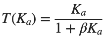
Before running the “3. Verify relative changes” code in the practice Live Script, calculate by hand using $K_a=5000,\quad\beta=0.05,\quad\delta=0.1$ .
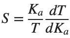
Differentiate $T(K_a)=\frac{K_a}{1+\beta K_a}$ and substitute into $S=\frac{K_a}{T}\frac{dT}{dK_a}$ to obtain the baseline sensitivity $S_0$ .
Approximate calculation: multiply $S_0$ by the relative increase 0.1 in $K_a$ .
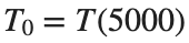
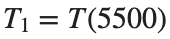
Exact calculation: Find $T_0=T(5000)$ and $T_1=T(5500)$ separately, then calculate $\frac{T_1-T_0}{T_0}$ .
You may leave both answers as fractions.
Save both handwritten calculations, then run the “3. Verify relative changes” code in the practice Live Script and compare them with approx·exact.
If they differ, check whether the denominator uses the pre-change $T_0$ .
Then repeat for the 1% and 20% conditions.
You have already completed the 10% condition, so you do not need to repeat it.

Before execution — Hand-calculated expressions and values: ⟦write calculations here⟧ After execution — MATLAB output values to compare: ⟦write output values here⟧

2. Baseline gain and sensitivity

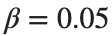
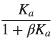
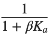
Sensitivity is the ratio of relative changes for a very small gain change. For a finite change such as +10%, the predicted change may differ slightly from recalculating the original function. Differentiating the overall gain T=Ka/(1+beta*Ka) gives dT/dKa=1/(1+beta*Ka)^2. Substituting into S=(Ka/T)*(dT/dKa) gives S=1/(1+beta*Ka). For a small change, ΔT≈(dT/dKa)ΔKa, hence ΔT/T≈S*(ΔKa/Ka). Below, approx uses this expression, while exact directly compares T before and after the change.

Prediction before running: ⟦enter here⟧

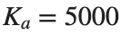
Ka=5000;beta=.05;
Topen=Ka;Tclosed=Ka/(1+Ka*beta);
Sopen=1;Sclosed=1/(1+Ka*beta);
disp(table(Topen,Tclosed,Sopen,Sclosed));

Do it yourself:

Keep

\beta=0.05

and apply

K_a\in\{1000,5000,10000\}

. Substitute each

K_a

into the open-loop gain

K_a

, closed-loop gain

\frac{K_a}{1+\beta K_a}

, and sensitivity

\frac1{1+\beta K_a}

, and tabulate the three gain conditions as rows.

% ✍ Your code: add your own code below.

Changed condition: ⟦enter here⟧

Observed result: ⟦enter here⟧

Differences from the prediction and their causes: ⟦enter here⟧

3. Verify relative changes

The relative change is (gain after change−gain before change)/gain before change. Check that you are not dividing by the changed gain.

Prediction before running: ⟦enter here⟧

Ka=5000;beta=.05;delta=.1;
T0=Ka/(1+Ka*beta);T1=(Ka*(1+delta))/(1+Ka*(1+delta)*beta);
exact=(T1-T0)/T0;approx=delta/(1+Ka*beta);
disp(table(exact,approx));

Do it yourself:

Calculate exact and approx in the relative-change calculation code for $\delta\in\{0.01,0.1,0.2\}$ . Keep $K_a=5000$ and $\beta=0.05$ unchanged.
Record δ, the exact relative change, the approximate relative change, and their absolute difference in one table.
Use the last table column to determine whether approximation error increases as δ increases. Also compare the relative gain change without feedback δ with the closed-loop value exact, and explain how much the change is reduced.

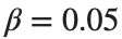
% ✍ Your code: add your own code below.

Changed condition: ⟦enter here⟧

Observed result: ⟦enter here⟧

Differences from the prediction and their causes: ⟦enter here⟧

4. Repeat the checks

Change Ka successively, calculate using the same sensitivity equation, and plot the curves. Check how sensitivity changes as Ka increases.

Prediction before running: ⟦enter here⟧

beta=.05;Ka=logspace(1,5,100);S=1./(1+Ka*beta);
figure;semilogx(Ka,S);xlabel('Amplifier gain Ka');ylabel('Sensitivity');grid on;

Do it yourself:

Add $0.01$ and $0.1$ to $\beta=0.05$ in the sensitivity plotting code. Plot three sensitivity curves on the same Ka vector and show β in the legend.
At the same $K_a$ , record the closed-loop gain and sensitivity for each β side by side. For example, compare the three cases at the baseline $K_a=5000$ .
Explain closed-loop gain in terms of output magnitude, and sensitivity in terms of the relative gain change caused by changes in $K_a$ . Distinguish a small gain from insensitivity to change.

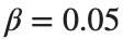
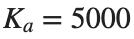
% ✍ Your code: add your own code below.

Changed condition: ⟦enter here⟧

Observed result: ⟦enter here⟧

Differences from the prediction and their causes: ⟦enter here⟧

Practice through repetition and check before submission

Summarize the three conditions compared in the preceding hands-on activities below. You do not need to repeat experiments already completed. Predictions may state increasing or decreasing trends instead of exact values.

Repetition 1 — Condition: ⟦enter here⟧ / Prediction: ⟦enter here⟧ / Actual result: ⟦enter here⟧

Trial 2 — Condition: ⟦enter here⟧ / Prediction: ⟦enter here⟧ / Observation: ⟦enter here⟧

Trial 3 — Condition: ⟦enter here⟧ / Prediction: ⟦enter here⟧ / Observation: ⟦enter here⟧

Optional:

Example: using matrix division instead of element-wise division

In a copy of the “4. Repeat the checks” code in the practice Live Script, replace S=1./(1+Ka*beta) with S=1/(1+Ka*beta). Record whether a vector Ka causes an error or yields dimensions different from those expected.
Change only this line to ./ and write size(Ka) and size(S). Check whether the two vectors' elements correspond one to one.

Include code, actual outputs and plots, and your own interpretation. Submit through KLAS; check the semester schedule and latest announcements for the deadline.

Filename: Name_StudentID_Week9.mlx.