
Control Engineering I · Week 10 · DC Motor Disturbance Rejection
English translation
Edit the code and response fields in your own copy. Name: ⟦enter here⟧ / Student ID: ⟦enter here⟧
How to run
In Live Editor, click inside the code and run the current section with Run Section (Windows/Linux Ctrl+Enter, Mac ⌘+Enter). Run executes the entire document. Edit the explanations and response fields directly.
Initially run from the top, and rerun any section whose values you change. If an undefined-variable error occurs, run the preceding sections first. Outputs appear below or to the right of the code.
Environment: MATLAB Online and Control System Toolbox.
1. Derive the model and calculate gain
- (input): Disturbance Torque.
- ω (output): Angular velocity deviation from the operating point [rad/s].
- : change in armature voltage.
- i: Change in armature current.
- Model assumption: Neglect armature inductance.


Symbol | Meaning | Value |
|---|---|---|
Armature Resistance | 1 | |
Torque Constant | 0.1 | |
Back EMF Constant | 0.1 | |
J | Moment of Inertia | 0.01 |
b | Viscous Friction Coefficient | 0.001 |
Tachometer Gain | 0.05 |


Motor equations:
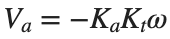
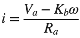
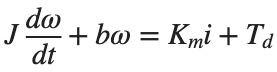
- Substitute the expression for into the expression for current i. Then substitute the resulting expression for i into the equation of motion, and rearrange as a differential equation relating ω and .
- Set the initial conditions to 0 and apply the Laplace transform to this differential equation. Collect terms containing on one side, then find .
- Record the numerator and denominator of your derived transfer function as separate coefficient arrays, in descending powers.


Find: The minimum amplifier gain satisfying the tolerance condition.
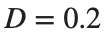
- Constant disturbance: .
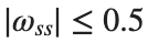
- Steady-state tolerance: rad/s.
- Amplifier gain range: .
- Motor coefficients: values in the table above.
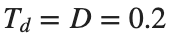

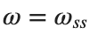
- Substitute , , and into the differential equation derived above. Divide both sides by the coefficient of to express as a function of .
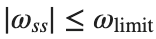
- Substitute that expression into the tolerance condition . Insert , , and the motor coefficients from the table, and find the range of that satisfies the condition.
- Record the smallest value in the range you found as . Include the expression for , the inequality with numerical values substituted, and the allowed range and minimum of . Use this record for the later comparison with MATLAB calculations.




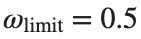


Before execution — Hand-calculated expressions and values: ⟦write calculations here⟧ After execution — MATLAB output values to compare: ⟦write output values here⟧
2. Open-loop Disturbance Step Response
The baseline is Ra=1,Km=Kb=0.1,J=0.01,b=0.001.
Prediction before running: ⟦enter here⟧
Ra=1;Km=.1;Kb=.1;J=.01;b=.001;D=.2;
Gd=tf(1,[J b+Km*Kb/Ra]);
finalValue=D*dcgain(Gd);disp(finalValue);
figure;step(D*Gd,0:.01:8);grid on;
Do it yourself:
Use Gd=tf(1,[J b+Km*Kb/Ra]) defined in the Open-loop Disturbance Step Response code. Keep Ra,Km,Kb,J,b at the values defined there.
Condition | D |
|---|---|
1 | 0.1 |
2 | 0.2 |
3 | 0.3 |
- For each condition, calculate [rad/s].
- Record the following three columns in one table.

- D
- [rad/s]


- Compare across the three rows. State whether the ratio is constant and how this result demonstrates proportionality between D and .


% ✍ Your code: add your own code below.
Changed condition: ⟦enter here⟧
Observed result: ⟦enter here⟧
Differences from the prediction and their causes: ⟦enter here⟧
3. Disturbance rejection with tachometer feedback
Use the positive disturbance direction as the reference.
Prediction before running: ⟦enter here⟧
Ra=1;Km=.1;Kb=.1;J=.01;b=.001;Kt=.05;D=.2;Ka=20;
Go=tf(1,[J b+Km*Kb/Ra]);Gc=tf(1,[J b+Km/Ra*(Kt*Ka+Kb)]);
figure;step(D*Go,D*Gc,0:.005:8);legend('Open-loop disturbance','Feedback disturbance');grid on;
disp([D*dcgain(Go),D*dcgain(Gc)]);
Do it yourself:
Keep Ra,Km,Kb,J,b,Kt and in the disturbance-rejection code with tachometer feedback unchanged; change only .
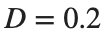

Condition | |
|---|---|
1 | 10 |
2 | 20 |
3 | 40 |

- For each , rebuild Gc and find dcgain(Gc).
- Multiply each DC gain by D to find [rad/s].
- Record , DC gain, and in three columns.
- Compare the symbolic coefficient arrays derived in activity 1 with the coefficient expressions written in this activity’s code.
- Find the first and second arguments of the tf call defining Gc, and record them as the numerator and denominator coefficient arrays, respectively.
- For each representation, divide its entire numerator and denominator by its leading denominator coefficient so that this coefficient becomes 1.
- Use two rows (numerator and denominator) and three columns (derived array, code array, and whether they agree). Compare coefficients at the same power and mark any differing terms.


% ✍ Your code: add your own code below.
Changed condition: ⟦enter here⟧
Observed result: ⟦enter here⟧
Differences from the prediction and their causes: ⟦enter here⟧
4. Design the amplifier gain
If decimal values are allowed for Ka, use the calculated minimum. If only integers are allowed, use the smallest integer no smaller than that value.
Prediction before running: ⟦enter here⟧
Ra=1;Km=.1;Kb=.1;b=.001;Kt=.05;D=.2;limit=.5;
Ka_min=max(0,(abs(D)/limit-b-Km*Kb/Ra)/(Km*Kt/Ra));
disp([Ka_min,ceil(Ka_min)]);
Do it yourself:
Keep and the motor coefficients from the preceding activity. Apply each of the two tolerances below.
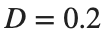
- First calculate the minimum gain using and limit=0.5 from your hand calculation. In the amplifier gain design code, Ka_min is the calculated value of . Record this output beside the value found by hand in activity 1.
- Calculate the minimum for each limit. The calculated corresponds to Ka_min in the code; decimal gains are allowed.
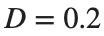


Condition | limit [rad/s] |
|---|---|
1 | 0.25 |
2 | 1 |
- Choose one slightly below and one above the minimum you found. Examples: , .
- Substitute each gain into the feedback model Gc, rebuild the model, and find .
- Record the calculations for all conditions in one table.


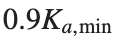
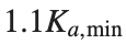

Tolerance [rad/s] | limit |
Calculated minimum gain | |
Gain applied to the model | |
Steady-state angular velocity deviation [rad/s] | |
Tolerance satisfied? | : true/false |


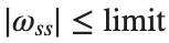
- Describe how gains below and above the minimum differ in meeting the tolerance. Use this table to judge whether the calculated minimum separates the two cases.
% ✍ Your code: add your own code below.
Changed condition: ⟦enter here⟧
Observed result: ⟦enter here⟧
Differences from the prediction and their causes: ⟦enter here⟧
Practice through repetition and check before submission
Summarize the three conditions compared in the preceding hands-on activities below. You do not need to repeat experiments already completed. Predictions may state increasing or decreasing trends instead of exact values.
Repetition 1 — Condition: ⟦enter here⟧ / Prediction: ⟦enter here⟧ / Actual result: ⟦enter here⟧
Trial 2 — Condition: ⟦enter here⟧ / Prediction: ⟦enter here⟧ / Observation: ⟦enter here⟧
Trial 3 — Condition: ⟦enter here⟧ / Prediction: ⟦enter here⟧ / Observation: ⟦enter here⟧
Optional:
Example: treating the last simulation sample as a steady-state value
- Keep the motor coefficients Ra,Km,Kb,J,b,Kt at their values from the preceding activity. Set Ka=20 and D=0.2, create Gc=tf(1,[J b+Km/Ra*(Kt*Ka+Kb)]), then find the last value of step(D*Gc,0:0.005:0.05).
- Record that value beside D*dcgain(Gc) and calculate the difference. Determine whether convergence is sufficient at 0.05 s.
- For the same Gc, increase the end time from 0.05 s to 8 s, keeping the time step at 0.005 s. Run [y_long,t_long]=step(D*Gc,0:0.005:8), then find the difference between y_long(end) and D*dcgain(Gc). Compare it with the earlier difference at 0.05 s.
Include code, actual outputs and plots, and your own interpretation. Submit through KLAS; check the semester schedule and latest announcements for the deadline.
Filename: Name_StudentID_Week10.mlx.