Control Engineering I · Week 03 · From Linearity to the Laplace Transform

English translation

Edit the code and response fields in your own copy. Name: ⟦enter here⟧ / Student ID: ⟦enter here⟧

How to run

In Live Editor, click inside the code and run the current section with Run Section (Windows/Linux Ctrl+Enter, Mac ⌘+Enter). Run executes the entire document. Edit the explanations and response fields directly.

Initially run from the top, and rerun any section whose values you change. If an undefined-variable error occurs, run the preceding sections first. Outputs appear below or to the right of the code.

Environment: MATLAB Online. With Symbolic Math Toolbox, use automatic transforms; otherwise, verify the partial-fraction solution below.

1. Counterexample to linearity

Substituting specific values lets you find cases that do not satisfy the linearity conditions.

Prediction before running: ⟦enter here⟧

x1=1;x2=2;
f=@(x)x.^2;
disp([f(x1+x2),f(x1)+f(x2)]);

Do it yourself:

Determine the linearity and time invariance of

3x

x^2

3x+1

\cos(t)x

, and

\frac{dx}{dt}

, and explain your reasoning for each.

% ✍ Your code: add your own code below.

Changed condition: ⟦enter here⟧

Observed result: ⟦enter here⟧

Differences from the prediction and their causes: ⟦enter here⟧

2. Linear Approximation

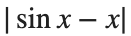
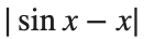
Calculate in radians.

Prediction before running: ⟦enter here⟧

x=linspace(-pi,pi,401);
figure;plot(x,sin(x),x,x);ylim([-2 2]);legend('sin(x)','linear approximation');grid on;
xlabel('x (rad)');ylabel('value');

Do it yourself:

Keep the notebook's x range and spacing, and calculate $|\sin x-x|$ at each x. Select samples whose error is at most $0.01$ , then write the endpoint x values of the contiguous interval containing 0.
At $x\in\{0.1,0.5,1\}$ rad, tabulate $\sin x$ , the approximation x, the absolute error $|\sin x-x|$ , and whether the tolerance condition is satisfied.

% ✍ Your code: add your own code below.

Changed condition: ⟦enter here⟧

Observed result: ⟦enter here⟧

Differences from the prediction and their causes: ⟦enter here⟧

3. Laplace Transform

With Symbolic Math Toolbox, calculate the transform and inverse. Without it, numerically verify the provided partial-fraction solution. These are two ways to check the same mathematical relationship.

Prediction before running: ⟦enter here⟧

if ~isempty(which('syms'))
    syms t s
    disp(laplace(exp(-5*t),t,s));
    disp(laplace(sin(3*t),t,s));
    X=12/(s*(s^2+5*s+6));
    x=ilaplace(X,s,t);disp(simplify(x));
    assert(isAlways(simplify(diff(x,t,2)+5*diff(x,t)+6*x-12)==0));
else
 % Without the Toolbox: substitute the solution obtained by partial fractions into the original ODE.
    disp('Transform: exp(-5t) -> 1/(s+5), sin(3t) -> 3/(s^2+9)');
    t=0:.01:5;
    x=2-6*exp(-2*t)+4*exp(-3*t);
    dx=12*exp(-2*t)-12*exp(-3*t);
    ddx=-24*exp(-2*t)+36*exp(-3*t);
    assert(max(abs(ddx+5*dx+6*x-12))<1e-10);
    assert(abs(x(1))<1e-10 && abs(dx(1))<1e-10);
    figure;plot(t,x);xlabel('Time (s)');ylabel('x(t)');grid on;
end

Do it yourself:

u(t)

is a unit step that changes from 0 to 1 at

t=0

and stays there.

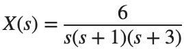
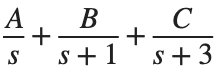
Check the transform and inverse transform of $e^{-2t}$ and sin(4t), then solve $\ddot x+4\dot x+3x=6u(t)$ with all initial conditions at 0.
Verify the solution by substituting it into the original equation.
Without the toolbox, decompose $X(s)=\frac6{s(s+1)(s+3)}$ into $\frac As+\frac B{s+1}+\frac C{s+3}$ to find the coefficients, then write the solution and its derivative in exponential form yourself and verify them.

% ✍ Your code: add your own code below.

Changed condition: ⟦enter here⟧

Observed result: ⟦enter here⟧

Differences from the prediction and their causes: ⟦enter here⟧

Practice through repetition and check before submission

Summarize the three conditions compared in the preceding hands-on activities below. You do not need to repeat experiments already completed. Predictions may state increasing or decreasing trends instead of exact values.

Repetition 1 — Condition: ⟦enter here⟧ / Prediction: ⟦enter here⟧ / Actual result: ⟦enter here⟧

Trial 2 — Condition: ⟦enter here⟧ / Prediction: ⟦enter here⟧ / Observation: ⟦enter here⟧

Trial 3 — Condition: ⟦enter here⟧ / Prediction: ⟦enter here⟧ / Observation: ⟦enter here⟧

Optional:

Example: Passing a value in degrees to a radian input

Examine using sin(30) to calculate the sine of 30°. Record this result and sind(30).
If keeping sin, change the input line to sin(pi/6). Record the values before and after the change and the input unit.

Include code, actual outputs and plots, and your own interpretation. Submit through KLAS; check the semester schedule and latest announcements for the deadline.

Filename: Name_StudentID_Week3.mlx.