Control Engineering I Week 2 Exercise — Physical Models and Responses

English translation

Run your own copy and record observations.

Follow predict → run → observe → explain physically in this exercise. Consult the self-study HTML for the circuit and mechanical model equations. Complete the blank fields in your own words.

Follow the teaching assistant's assignment instructions for the submission filename and format.

Before starting · How to run sections

Click inside the code and use Run Section in Live Editor to run the entire current section.

Run a section: Windows/Linux Ctrl+Enter, Mac ⌘+Enter, or the Run Section button. Run executes the entire document.

Start in this order: check the environment → run the RLC baseline → change one RLC variable at a time → mechanical model. Fill in each prediction field first, run with Run Section, then observe the results.

Rerun sections where you changed parameter or factor. Outputs appear to the right of or below the code. Fill in the explanation blanks and tables yourself.

If variables such as R0 or g0 are missing, run sections in order from the RLC baseline section. In a new session, also run from the top and save your own copy.

Check first

The code below displays the MATLAB version and checks the required functions. Control System Toolbox is required. If tf cannot be found, ask the teaching assistant to check the environment.

disp(version);
assert(exist('tf','file') ~= 0, 'Control System Toolbox의 tf 함수를 확인하세요.');

1. Derive the physical model

Perform the calculations below first, then compare with MATLAB results.

Input

u(t)

is external force [N], and output

y(t)

is mass displacement [m].

Use $M=1,\ b=2,\ k=5$ for the mechanical model.
Before running the code, mark the force directions and derive the differential equation using Newton's law.
Set the initial conditions to 0, apply the Laplace transform to find $\frac{Y(s)}{U(s)}$ , then calculate the final displacement under a constant force of 1 N.
Compare MATLAB's transfer function and final response with your own equations.
Record this calculation in the prediction field for the baseline case among the three mechanical-model comparisons.

Before execution — Hand-calculated expressions and values: ⟦write calculations here⟧ After execution — MATLAB output values to compare: ⟦write output values here⟧

2. Baseline response of the parallel RLC circuit

The input is current [A], and the output is voltage [V]. With all initial conditions at 0, the transfer function has numerator s and denominator C*s^2 + (1/R)*s + 1/L.

Prediction before running: What will the voltage be initially and after a long time? Response: ______

R0 = 0.5; % ohm
L0 = 1;   % H
C0 = 5;   % F
t_rlc = linspace(0,25,1001);
g0 = tf([1 0], [C0 1/R0 1/L0]);
disp(g0);
figure('Name','RLC baseline');
step(g0,t_rlc);
grid on;
title('Parallel RLC: 1 A current step');
xlabel('Time (s)'); ylabel('Voltage (V)');

Observation: Describe what matches or differs from your prediction. Write: ______

Write coefficient arrays in descending powers of s. Omitting the final 0 in numerator [1 0] produces a different model.

Change R, L, and C one at a time

The baseline values are

R=0.5

Ω,

L=1

H, and

C=5

F. The input is current [A], and the output is voltage [V].

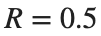
Run the baseline model’s unit-step response, then set parameter to "R", "L", and "C" in turn. For each parameter, rerun the “Change R, L, and C one at a time” code in the practice Live Script with factor=2 and factor=0.5. Keep the two unselected parameters at their baseline values.
Compare peak voltage, oscillation, and convergence between baseline and modified curves for each run. Record the changed parameter, its values before and after the change, and observed differences in the corresponding observation-table row.
For each parameter, explain one observed change in relation to the roles of resistance, inductance, and capacitance. Include a legend identifying conditions and units for time and voltage in the plot.

parameter = "R"; % Student changes: "R", "L", "C"
factor = 1;      % Student changes: 2 or 0.5
assert(any(parameter == ["R","L","C"]), 'parameter는 R, L, C 중 하나여야 합니다.');
assert(isscalar(factor) && isfinite(factor) && factor > 0, 'factor는 양수여야 합니다.');
R = R0; L = L0; C = C0;
switch parameter
 case "R"
        R = R0*factor;
 case "L"
        L = L0*factor;
 case "C"
        C = C0*factor;
end
g_changed = tf([1 0], [C 1/R 1/L]);
figure('Name','RLC comparison');
step(g0,g_changed,t_rlc);
grid on;
legend('Baseline',char(parameter + " x " + string(factor)), 'Location','best');
title('Change one parameter');
xlabel('Time (s)'); ylabel('Voltage (V)');

Use the table below to organize your observations. Fill each row after performing its corresponding experiment. Label any saved graphs with the parameter values.

Change	Prediction before execution	Plot observations	Physical explanation
R x 2	Not filled in	Not filled in	Not filled in
R x 0.5	Not filled in	Not filled in	Not filled in
L x 2	Not filled in	Not filled in	Not filled in
L x 0.5	Not filled in	Not filled in	Not filled in
C x 2	Not filled in	Not filled in	Not filled in
C x 0.5	Not filled in	Not filled in	Not filled in

Interpretation hint: Separate what changes from what stays fixed. Consider resistance effects in today's parallel circuit.

3. Baseline response of the mass–spring–damper

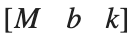
The input is force [N], and the output is displacement from equilibrium [m]. The equation is My'' + by' + k*y = u. The numerator is 1, and the denominator coefficients are [M b k].

Prediction before execution: Will displacement keep increasing under a continuously applied constant force? Write: ______

M = 1; b = 2; k = 5;
t_msd = linspace(0,15,1001);
g_msd = tf(1,[M b k]);
figure('Name','Mechanical baseline');
step(g_msd,t_msd);
grid on;
title('Mass-spring-damper: 1 N force step');
xlabel('Time (s)'); ylabel('Displacement (m)');

Observations and reasons: Response: ______

Compare three cases on one plot

The row order for each condition is

\left[\begin{array}{ccc}M&b&k\end{array}\right]

Condition	M	b	k
Baseline	1	2	5
Increased damping	1	8	5
Increase spring stiffness	1	2	10

Keep the first row of cases, change the second row to [1 8 5], and the third to [1 2 10]. Run the three responses with the same 1 N step input and time axis.
Place all three curves in one figure, with a legend identifying the conditions and units for time and displacement. In the observation table, describe how peak displacement, presence of oscillations, convergence, and final displacement differ from the baseline curve.
Relate increased damping to the role of b and increased spring stiffness to the role of k. Explain the difference in final displacement using the steady-state force relationship.

cases = [1 2 5;
         1 2 5;  % Student changes: increased damping
         1 2 5]; % Student changes: increased spring stiffness
assert(isequal(size(cases),[3 3]) && all(cases(:)>0), 'cases는 양수의 3x3 배열이어야 합니다.');
figure('Name','Mechanical comparison');
hold on;
for idx = 1:3
    g_case = tf(1,cases(idx,:));
    [y_case,time_case] = step(g_case,t_msd);
    plot(time_case,y_case,'LineWidth',1.5);
end
hold off;
grid on;
legend('Case 1','Case 2','Case 3','Location','best');
title('Compare the three cases');
xlabel('Time (s)'); ylabel('Displacement (m)');

Case	Observations about the final value	Observations on oscillation and peaks	Observations on settling time
Case 1	Not filled in	Not filled in	Not filled in
Case 2	Not filled in	Not filled in	Not filled in
Case 3	Not filled in	Not filled in	Not filled in

Explanation: Does greater damping always mean faster settling? Does a stiffer spring give the same final value? Explain using the graphs and model equations. Write: ______

Check before saving and submitting

Have you recorded the result and physical meaning of each RLC parameter change?
Are the mechanical-model comparison conditions (M,b,k)=(1,2,5), (1,8,5), (1,2,10)?
Are all three cases shown on one plot with readable legends and units?
Have you completed unfinished fields and explained the results in your own words?
Is your work saved, and does your submission method follow the teaching assistant's instructions?

KLAS Week 2 assignment deadline: 2026-09-10 23:59. Follow the latest announcement if it changes.

Submission deadline: 2026-09-10 23:59 (Korean time) Submission filename and format: Follow the teaching assistant's submission instructions. Submission location: The corresponding KLAS assignment. Follow the latest announcement if changes are posted.