Control Engineering I · Week 05 · Select States to Build a Matrix Model

English translation

Edit the code and response fields in your own copy. Name: ⟦enter here⟧ / Student ID: ⟦enter here⟧

How to run

In Live Editor, click inside the code and run the current section with Run Section (Windows/Linux Ctrl+Enter, Mac ⌘+Enter). Run executes the entire document. Edit the explanations and response fields directly.

Initially run from the top, and rerun any section whose values you change. If an undefined-variable error occurs, run the preceding sections first. Outputs appear below or to the right of the code.

Environment: MATLAB Online and Control System Toolbox.

1. Derive the state equations

Perform the calculations below first, then compare with MATLAB results.

R, L, and C are connected in parallel between the same two nodes. Take the lower node as the reference potential. Define the upper-node voltage as v, the downward inductor current as $i_L$ , and the supply current as u.
In $R=1,\ L=1,\ C=1$ , use KCL and $v=L\frac{di_L}{dt}$ to write the two differential equations for $\mathbf x=[v,i_L]^T$ and the output $y=v$ yourself, and find $A,B,C,D$ .
Set the initial conditions to 0 and apply the Laplace transform to both equations. In the inductor relation, express $I_L(s)$ in terms of $V(s)$ , then substitute it into the KCL equation. Collect terms containing $V(s)$ to find $\frac{V(s)}{U(s)}$ .
First state the values of v and $i_L$ after supplying a constant current of 1 A for a sufficiently long time.
Create an ss model using the matrices you derived and verify using tf·dcgain.
This parallel circuit differs in configuration from the circuit with a series RL branch below.
For this activity, replace one of the three repeated R values for the RL circuit with this comparison.

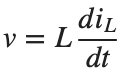
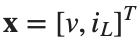
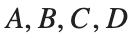
Before execution — Hand-calculated expressions and values: ⟦write calculations here⟧ After execution — MATLAB output values to compare: ⟦write output values here⟧

2. Mechanical State Space

Rebuild the baseline model each time without using a function.

Prediction before running: ⟦enter here⟧

M=1;b=2;k=5;
A=[0 1;-k/M -b/M];B=[0;1/M];Cout=[1 0];D=0;
sys=ss(A,B,Cout,D);disp(size(A));disp(tf(sys));
figure;step(sys,10);grid on;
assert(abs(dcgain(sys)-1/k)<1e-10);

Do it yourself:

Keep the mechanical model's $M=1$ and $k=5$ , and rebuild A and sys for $b\in\{0.5,2,10\}$ . Plot the three position step responses on the same time axis and label b in the legend.
Compare the presence of oscillations and convergence of each curve. State which b curve supports your judgment.
Using the same state order, select only linear velocity as the output. Record the Cout and dcgain(sys) used beside their values for position output.

% ✍ Your code: add your own code below.

Changed condition: ⟦enter here⟧

Observed result: ⟦enter here⟧

Differences from the prediction and their causes: ⟦enter here⟧

3. Electrical State Space

The input is a current source, with an RL branch in parallel with a capacitor, and the output is the resistor voltage.

Prediction before running: ⟦enter here⟧

R=3;L=1;Ccap=.5;
A=[0 -1/Ccap;1/L -R/L];B=[1/Ccap;0];Cout=[0 R];D=0;
sys=ss(A,B,Cout,D);
figure;step(sys,15);grid on;
assert(abs(dcgain(sys)-R)<1e-10);

Do it yourself:

The states of this circuit are

x=\left[\begin{array}{cc}v_C&i_L\end{array}\right]^{\mathsf T}

v_C

is the capacitor voltage [V], and

i_L

is the current in the series RL branch [A].

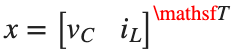
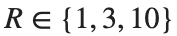
Keep the baseline circuit's other coefficients unchanged and, at $R\in\{1,3,10\}$ , rebuild A, Cout, and sys.
Calculate the final output voltage for a 1 A input using dcgain(sys), and record R and voltage in two columns.
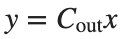
State that Ccap is capacitance and Cout is the output matrix. Use the state order and Cout to write the output equation $y=C_{\mathrm{out}}x$ , and determine whether it represents the desired resistor voltage.

% ✍ Your code: add your own code below.

Changed condition: ⟦enter here⟧

Observed result: ⟦enter here⟧

Differences from the prediction and their causes: ⟦enter here⟧

4. State coordinates and initial values

Nonzero initial position and velocity produce a response even without an input.

Prediction before running: ⟦enter here⟧

sys=ss([0 1;-5 -2],[0;1],[1 0],0);
figure;initial(sys,[1;0],0:.01:10);grid on;

Do it yourself:

On the same time axis as the baseline model, plot initial(sys,[0;1],0:0.01:10) and initial(sys,[1;0],0:0.01:10). Label the initial states in the legend.
State which state starts at a value other than 0 and whether an external input is present. Distinguish the step response with initial state 0 from the output caused by the initial state.

% ✍ Your code: add your own code below.

Changed condition: ⟦enter here⟧

Observed result: ⟦enter here⟧

Differences from the prediction and their causes: ⟦enter here⟧

Practice through repetition and check before submission

Summarize the three conditions compared in the preceding hands-on activities below. You do not need to repeat experiments already completed. Predictions may state increasing or decreasing trends instead of exact values.

Repetition 1 — Condition: ⟦enter here⟧ / Prediction: ⟦enter here⟧ / Actual result: ⟦enter here⟧

Trial 2 — Condition: ⟦enter here⟧ / Prediction: ⟦enter here⟧ / Observation: ⟦enter here⟧

Trial 3 — Condition: ⟦enter here⟧ / Prediction: ⟦enter here⟧ / Observation: ⟦enter here⟧

Optional:

Example: Selecting the wrong state as the output

Keep A,B,D of the mechanical model unchanged. When position is required, record the transfer functions obtained using Cout=[0 1] and Cout=[1 0].
State the order of the states and the units of each output. Change only the Cout line to output position, and rebuild the model.

Include code, actual outputs and plots, and your own interpretation. Submit through KLAS; check the semester schedule and latest announcements for the deadline.

Filename: Name_StudentID_Week5.mlx.