
Control Engineering I · Week 04 · Connecting Transfer Functions and Blocks
English translation
Edit the code and response fields in your own copy. Name: ⟦enter here⟧ / Student ID: ⟦enter here⟧
How to run
In Live Editor, click inside the code and run the current section with Run Section (Windows/Linux Ctrl+Enter, Mac ⌘+Enter). Run executes the entire document. Edit the explanations and response fields directly.
Initially run from the top, and rerun any section whose values you change. If an undefined-variable error occurs, run the preceding sections first. Outputs appear below or to the right of the code.
Environment: MATLAB Online and Control System Toolbox. Simulink is also required to run the Simulink model.
1. Construct the transfer function
Enter coefficients in descending powers.
Prediction before running: ⟦enter here⟧
G=tf(1,[1 2 5]);
T=feedback(G,1);
disp(G);disp(T);
assert(abs(dcgain(G)-.2)<1e-10);
Do it yourself:
- Substitute , , and into the mechanical model's transfer function to create a MATLAB model.
- Write the transfer function used and record dcgain(G) beside the hand-calculated . State whether the two values agree.




% ✍ Your code: add your own code below.
Changed condition: ⟦enter here⟧
Observed result: ⟦enter here⟧
Differences from the prediction and their causes: ⟦enter here⟧
2. Block connections and responses
Compare using the same time axis.
Prediction before running: ⟦enter here⟧
G=tf(1,[1 2 5]);T=feedback(G,1);t=0:.01:10;
figure;step(G,T,t);legend('Open-loop','Unity feedback');grid on;
Do it yourself:
- Keep the baseline G=tf(1,[1 2 5]) and connect negative feedback with .
- Write the closed-loop transfer function simplified by hand beside the result of feedback(G,2).
- Write and compare the denominator coefficients of both equations in the same order of powers. Also mark which coefficients differ from the case .


% ✍ Your code: add your own code below.
Changed condition: ⟦enter here⟧
Observed result: ⟦enter here⟧
Differences from the prediction and their causes: ⟦enter here⟧
3. Open the Simulink model
Open the accompanying .slx in MATLAB Drive, or build the same model as shown below.
Prediction before running: ⟦enter here⟧
modelName='Control_Engineering_1_Week04_Block_Model';
if isfile([modelName '.slx'])
open_system(modelName);
else
disp('블로그 자료 모음에서 Week04 .slx 파일을 같은 폴더에 받으세요.');
end
Do it yourself:
- Connect Step → Transfer Fcn → Scope in Simulink. Set the numerator to [1] and denominator to [1 2 5] to match the baseline G=tf(1,[1 2 5]).
- Run with Step time=0, Final value=1, and Stop time=10.
- Present the Scope output beside MATLAB's step(G,0:0.01:10) curve. Use the same time range and output-axis range, and state whether the final values and curve shapes agree. This block diagram corresponds to G without feedback.
% ✍ Your code: add your own code below.
Changed condition: ⟦enter here⟧
Observed result: ⟦enter here⟧
Differences from the prediction and their causes: ⟦enter here⟧
Practice through repetition and check before submission
Summarize the three conditions compared in the preceding hands-on activities below. You do not need to repeat experiments already completed. Predictions may state increasing or decreasing trends instead of exact values.
Repetition 1 — Condition: ⟦enter here⟧ / Prediction: ⟦enter here⟧ / Actual result: ⟦enter here⟧
Trial 2 — Condition: ⟦enter here⟧ / Prediction: ⟦enter here⟧ / Observation: ⟦enter here⟧
Trial 3 — Condition: ⟦enter here⟧ / Prediction: ⟦enter here⟧ / Observation: ⟦enter here⟧
Optional:
Example: changing the coefficient order in a transfer-function denominator
- Create the baseline tf(1,[1 2 5]) and a separate model tf(1,[5 2 1]) with reversed coefficient order.
- Write each denominator polynomial and DC gain side by side. Change only the denominator vector to [1 2 5] so that .
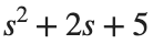
Include code, actual outputs and plots, and your own interpretation. Submit through KLAS; check the semester schedule and latest announcements for the deadline.
Filename: Name_StudentID_Week4.mlx.