

Frequency Response · Lesson
English translation
Execution conditions
MATLAB · Control System Toolbox
Topics covered
Understanding how amplitude and phase change at each frequency connects Bode plots to actual signals.
Overall workflow
Sinusoidal input → steady-state output → amplitude ratio and phase → Bode plot
Applying a sinusoid and examining only steady state
When sin(ωt) is applied to a linear system, the stable steady-state output is a sinusoid at the same frequency. The amplitude ratio is |G(jω)|, and the shift relative to the input is the phase.
Exclude the initial transient response from estimation.
Bode plot units
Gain in dB is 20log10(amplitude ratio). Check whether phase is in degrees or radians. Since 1 Hz equals 2π rad/s, substituting the number 1 directly gives a different experiment.
Near resonance, even a small frequency change can greatly affect the response.
Sinusoids and phase lag
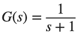
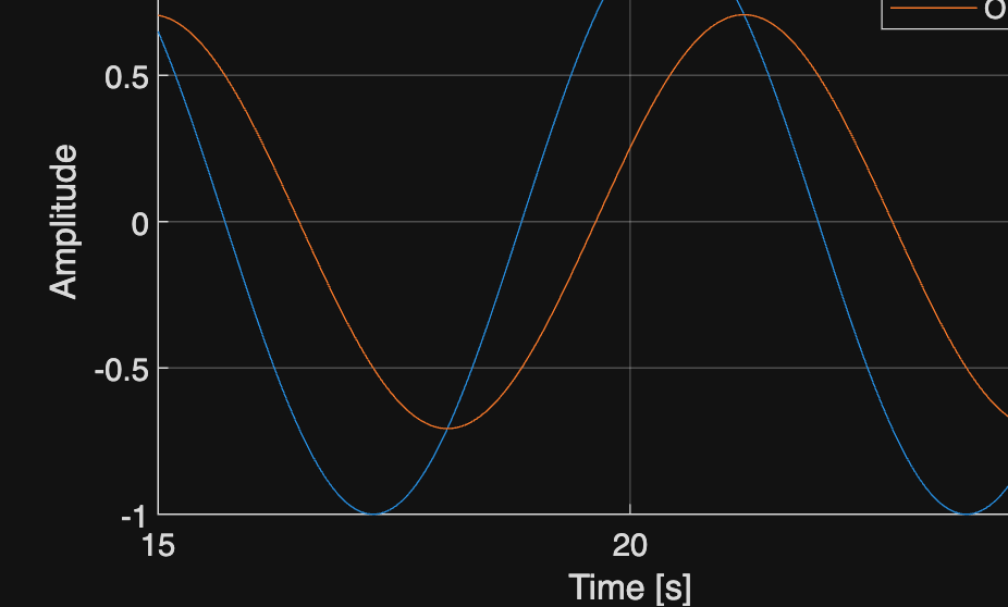
Apply sin(t) to . At rad/s, the amplitude ratio is 1/√2 and the phase is −45°.
%% Worked example
s=tf('s'); G=1/(s+1); t=linspace(0,25,2501)'; u=sin(t);
y=lsim(G,u,t); figure; plot(t,u,t,y); xlim([15 25]);
xlabel('Time [s]'); ylabel('Amplitude'); legend('Input','Output'); grid on
z=evalfr(G,1i); fprintf('Magnitude %.9g, Phase [deg] %.9g\n',abs(z),rad2deg(angle(z)));
Reference example
View more examples